Учебники / 0841558_16EA1_federico_milano_power_system_modelling_and_scripting

where vh is the generator bus voltage or any bus voltage regulated by the AVR, vm is the state variable used as voltage signal within the AVR and Tr the measurement block time constant. Equations (16.9)-(16.11) constitute the common equations of AVR models and can be included in a base AVR class.

The reference voltage v0ref is initialized after the power flow analysis and after the initialization of synchronous machines. In case the violations of AVR limits, the data of the static generator used in power flow analysis are not consistent with the AVR data and, thus, AVR state variables cannot be correctly initialized.

16.2.1Automatic Voltage Regulator Type I

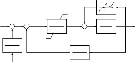
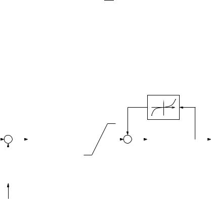
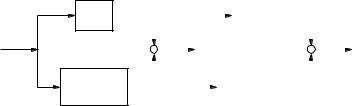
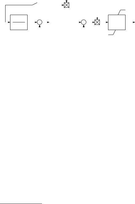
The AVR Type I depicted in Figure 16.8 represents a typical dc exciter model. The DAE system is (16.9)-(16.11) and:

where vh is the generator terminal voltage or a remote-bus regulated voltage and the ceiling function Se is:2

This model is a simplified version of the classic IEEE type DC1 [145]. The IEEE DC1 system includes an additional lead-lag block before the amplifier block. However, this lead-lag block is often neglected. The amplifier state variable vr1 is subjected to an anti-windup limit. Table 16.3 defines all parameters of AVR Type I.

2The coe cients Ae and Be can be determined by measuring two points of the ceiling function Se. Typically, one knows the values Semax and Se0.75·max that correspond to the field voltages vfmax and 0.75 · vfmax, respectively. To compute Ae and Be , one has to solve the following system:

0 = −(1 + Semax)vfmax + vrmax

Semax = AeeBe vfmax

Se0.75·max = AeeBe ·0.75·vfmax

where Semax, Se0.75·max, vfmax, and vrmax are given values.

Fig. 16.8 Automatic voltage regulator Type I control diagram

Table 16.3 Automatic voltage regulator Type I parameters

16.2.2Automatic Voltage Regulator Type II

The AVR Type II is shown in Figures 16.9 and 16.10. This AVR models a typical static exciter which is characterized by higher gains and faster response than the previous dc exciter. The DAE system is (16.9)-(16.11) and:

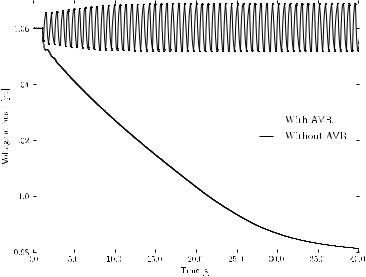
Example 16.2 E ect of Automatic Voltage Regulation on Synchronous Machine Bus Voltage

Figure 16.12 shows the e ect of the automatic voltage regulation on the bus voltage of synchronous machine 1 of the IEEE 14-bus system. The transient refers to line 2-4 outage at t = 1 s. As expected, the system without primary voltage regulation does not recover the desired voltage values after the disturbance.

Figure 16.14 shows the transient following the same disturbance but with a 20% load increase.3 For this loading level, the line outage leads to an unstable equilibrium point, as shown in Figure 16.13. In fact, as discussed in Example 8.9 of Chapter 8, a Hopf bifurcation occurs when increasing the loading level. In summary, the response of the system without AVRs is poor but, depending on the loading level, the inclusion of AVRs can lead to instability. Thus, it is required to include additional controllers to improve the system transient behavior. A solution is provided by power system stabilizers that are described in the following section.

3Loads are modelled as constant powers and are switched to constant impedances for low bus voltage magnitude, i.e., vh < 0.8 pu.

Fig. 16.14 E ect of automatic voltage regulation on synchronous machine bus voltage for the IEEE 14-bus system (120% loading level)

16.3Power System Stabilizer

Power System Stabilizers (PSSs) are used for damping power system oscillations. Although several PSS models have been proposed in the literature, the rationale behind the PSS functioning is the same for all control schemes. To explain the basic functioning of PSSs, consider a simple electromechanical model of the synchronous machine with no damping:

di erentiating the above expression and assuming a constant mechanical power pm leads to:

which has a pair of pure complex eigenvalues (no damping):

In practice (16.30) is obtained by introducing a feedback signal proportional to the active power or rotor frequency into the primary voltage control loop. Typical PSS input signals are the rotor speed ω, the active power ph and also the bus voltage vh of the generator to which the PSS is connected through the automatic voltage regulator. The PSS output signal is a signal vs that modifies the reference voltage vref of the AVR.

In the following subsections, four typical PSS models are described. Except for the simple model described in Subsection 16.3.1, other models have two algebraic equations, as follows:

where (16.35) defines the PSS signal vs, and (16.36) sums the signal vs to the AVR reference voltage (see also (16.10)). All PSS parameters used in the following subsections are defined in Table 16.6.