Учебники / 0841558_16EA1_federico_milano_power_system_modelling_and_scripting

whereas the link between voltages, currents and state variables is as follows:

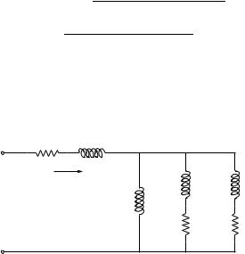
Fig. 15.14 Electrical circuit of the third-order induction machine model

15.2.5Detailed Double-Cage Model

The electrical circuit for the double-cage induction machine model is depicted in Figure 15.15. As for the single-cage model, real and imaginary axes are defined with respect to the network reference angle, and (15.60) and (15.61) apply. Two voltages behind the stator resistance rS model the cage dynamics, as follows:

352 15 Alternate-Current Machines

and the links between voltages and currents are:

where the parameters are determined from the circuit resistances and reactances and are given by equations (15.64) and:

T0 = xR2 + xR1xμ/(xR1 + xμ) ΩbrR2

The di erential equation for the slip is the (15.65), while the electrical torque is defined as follows:

Fig. 15.15 Electrical circuit of the fifth-order induction machine model

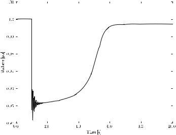
Example 15.7 Induction Motor Start-Up

Figure 15.16 shows the start-up of a double-cage induction motor modelled with a fifth order set of DAE as discussed in the previous section. The motor is connected to the network at t = 1 s. Fast electrical dynamics damp out in about a second while the mechanical transient takes several seconds. Thus, fast dynamics should be considered in the classical transient stability analysis i.e., for time scale from one to five seconds after the fault clearing. For voltage

Fig. 15.16 Induction motor start-up transient

or frequency stability analysis (e.g., tens of seconds), a simple mechanical model for the induction motor is adequate.

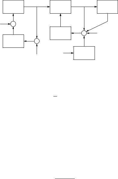
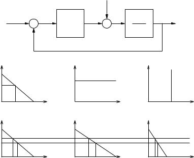
Fig. 16.2 Basic functioning of the primary frequency control: (a) linearized control loop; (b) e ect of the droop R on the control loop; and (c) e ect of a variation of the rotor speed Δω on a multi-machine system with Rj = 0, j G

Only the relative values of the coe cients γi are relevant, not the absolute ones. Two relevant remarks are as follows:

1.If Rk → ∞, γk = 0 for the machine k.

2.If Rk = 0, γk = 1 for the machine k, being all other loss participation coe cients γj = 0, j G and j = i.

When defining the TG data, the droop R and mechanical power limits are often given in pu with respect to the synchronous machine power rating. If this is the case, during the initialization of turbine governors data, the droops have to be converted to the system power base, as follows:

When initializing the turbine governor variable, mechanical power limits have to be checked. If a limit is violated, it means that the turbine governor parameters are not consistent with those of the static generator used in power flow analysis.

Each turbine governor model has two algebraic equations, as follows:

where (16.5) represents the link between the turbine governor and the synchronous machines, being τm the input mechanical power variable used in synchronous machine models, i.e., (16.5) substitutes (15.7); and (16.6) defines the turbine governor reference rotor speed. The reference signal ω0ref can be modified, for example, by the automatic generation control (e.g., secondary frequency regulation).

Following subsections describe two simple yet commonly used turbine governor models.

16.1.1Turbine Governor Type I

The TG type I is depicted in Figure 16.3. It includes a governor, a servo and a reheat block. The DAE system that describes this TG model is as follows:

The number of blocks of each part of the turbine can be increased to take into account each stage in detail. However, the structure of the control diagram does not change. Table 16.1 defines the parameters of TG type I.

Example 16.1 E ect of Turbine Governor on Generator Frequency

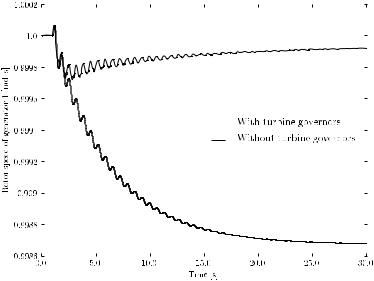
Figure 16.5 shows the e ect of turbine governors on generator rotor speeds for the IEEE 14-bus system. The plot was obtained including two turbine governors of type II at generators 1 and 2. The complete data are reported in Appendix D. The disturbance is line 2-4 outage at t = 1 s. As expected, the turbine governor is able to recover the rotor speed to a value close to the initial synchronous speed. However, since the disturbance considered in this case study implies only a redistribution of losses, the e ect of turbine governor is negligible.1 As discussed above, the primary frequency regulation is never integral, hence the final frequency cannot be equal to the initial one.

Turbine governors regulates the production of synchronous machine active powers. In the case of the IEEE 14-bus system, only two machines produce active power. Since synchronous machine 1 is ten times bigger than machine 2 and the two machines have the same droop, machine 1 takes about the 90% of the active power variation after the disturbance.

1In fact, without turbine governors, the frequency error is < 0.2%. This is why turbine governors are not considered in most examples of this book.

Fig. 16.5 E ect of the turbine governor on the generator frequency for the IEEE 14-bus system

16.2Automatic Voltage Regulator

Automatic Voltage Regulators (AVRs) define the primary voltage regulation of synchronous machines. Several AVR models have been proposed and realized in practice [89, 145]. In this section, three simple AVR types are described. AVR Type I is a simplified version of the standard dc exciter IEEE type I, whereas AVR Type II is a typical static exciter model. AVR Type III is the simplest AVR model that can be used for rough stability evaluations.

Figure 16.6 depicts a conceptual linearized model of the primary voltage regulation of the synchronous machine. Although the detailed system is much more complicated, the kernel of primary voltage regulation can be reduced to a transfer function composed of the AVR regulator, the exciter and the machine d-axis emf. The system of Figure 16.6 has the closed-loop root loci shown in Figure 16.7. Depending on the AVR gain the system can be stable or unstable (due to the occurrence of a Hopf bifurcation). Clearly, AVR gains are chosen to avoid instability in most operating conditions. However, it is possible that an unusual loading condition and/or line outage causes an increase of the equivalent closed-loop gain and, thus, leads to instability [337]. This phenomenon is illustrated in Example 16.2.