

Kleiber - Applied econometrics in R
.pdf184 7 Programming Your Own Analysis
set much more cumbersome. Therefore, R ships with support for tightly bundling R scripts (as discussed in (b)) and the documentation of their output so that R first runs the analysis and then includes the results in the documentation. Base R provides the function Sweave() (in package utils), which by default supports “weaving” of R code with LATEX documentation but also allows other documentation formats to be plugged in.
In the following, we provide examples for a few typical tasks in econometric analysis—simulation of power curves, bootstrapping a regression, and maximizing a likelihood. In doing so, we go beyond using o -the-shelf software and in each case require some of the steps discussed above.
7.1 Simulations
A simulation study is one of the most typical programming tasks when evaluating some algorithm; e.g., a test procedure or an estimator. It usually involves (at least) three steps: (1) simulating data from some data-generating process (DGP); (2) evaluating the quantities of interest (e.g., rejection probabilities, parameter estimates, model predictions); and (3) iterating the first two steps over a number of di erent scenarios. Here, we exemplify how to accomplish such a task in R by comparing the power of two well-known tests for autocorrelation—the Durbin-Watson and the Breusch-Godfrey test—in two di erent specifications of a linear regression. In the following, we first set up three functions that capture the steps above before we actually run the simulation and summarize the results both numerically and graphically.
Data-generating process
We consider the Durbin-Watson and Breusch-Godfrey tests for two di erent linear regression models: a trend model with regressor xi = i and a model with a lagged dependent variable xi = yi−1. Recall that the Durbin-Watson test is not valid in the presence of lagged dependent variables.
More specifically, the model equations are
trend: yi = β1 + β2 · i + "i, dynamic: yi = β1 + β2 · yi−1 + "i,
where the regression coe cients are in both cases β = (0.25, −0.75)>, and {"i}, i = 1, . . . , n, is a stationary AR(1) series, derived from standard normal innovations and with lag 1 autocorrelation %. All starting values, both for y and ", are chosen as 0.
We want to analyze the power properties of the two tests (for size = 0.05) on the two DGPs for autocorrelations % = 0, 0.2, 0.4, 0.6, 0.8, 0.9, 0.95, 0.99 and sample sizes n = 15, 30, 50.
To carry out such a simulation in R, we first define a function dgp() that implements the DGP above:
7.1 Simulations |
185 |
R> dgp <- function(nobs = 15, model = c("trend", "dynamic"),
+corr = 0, coef = c(0.25, -0.75), sd = 1)
+{
+model <- match.arg(model)
+coef <- rep(coef, length.out = 2)
+err <- as.vector(filter(rnorm(nobs, sd = sd), corr,
+method = "recursive"))
+if(model == "trend") {
+x <- 1:nobs
+y <- coef[1] + coef[2] * x + err
+} else {
+y <- rep(NA, nobs)
+y[1] <- coef[1] + err[1]
+for(i in 2:nobs)
+y[i] <- coef[1] + coef[2] * y[i-1] + err[i]
+x <- c(0, y[1:(nobs-1)])
+}
+return(data.frame(y = y, x = x))
+}
The arguments to dgp() are nobs (corresponding to n with default 15), model (specifying the equation used, by default "trend"), corr (the autocorrelation %, by default 0), coef (corresponding to β), and sd (the standard deviation of the innovation series). The latter two are held constant in the following. After assuring that model and coef are of the form required, dgp() sets up the regressor and dependent variable and returns both in a “data.frame” comprising the variables y and x.
Evaluation for a single scenario
Based on this implementation of the DGP, we can now easily simulate the power of both tests for a given combination of parameters. In simpower(), we just iterate through a for() loop (by default with nrep = 100 iterations) in which we simulate a data set, apply both dwtest() (the Durbin-Watson test from lmtest) and bgtest() (the Breusch-Godfrey test from lmtest) to it, and store the associated p values. After completing the for() loop, we return the proportion of significant p values (by default at size = 0.05).
R> simpower <- function(nrep = 100, size = 0.05, ...)
+{
+pval <- matrix(rep(NA, 2 * nrep), ncol = 2)
+colnames(pval) <- c("dwtest", "bgtest")
+for(i in 1:nrep) {
+dat <- dgp(...)
+pval[i,1] <- dwtest(y ~ x, data = dat,
186 7 Programming Your Own Analysis
+alternative = "two.sided")$p.value
+pval[i,2] <- bgtest(y ~ x, data = dat)$p.value
+}
+return(colMeans(pval < size))
+}
The remaining argument ... is a simple mechanism for passing on further arguments to other functions. Here, any argument beyond nrep and size is passed to dgp(). For example, we could easily modify the correlation employed via simpower(corr = 0.9), which would then internally call dgp(corr = 0.9), all other defaults remaining unchanged.
Iterated evaluation over all scenarios
Given these two building blocks, the DGP and the power simulator, we can now set up the main simulation routine in which we compute the power for di erent combinations of autocorrelation, sample size, and regression model:
R> simulation <- function(corr = c(0, 0.2, 0.4, 0.6, 0.8,
+0.9, 0.95, 0.99), nobs = c(15, 30, 50),
+model = c("trend", "dynamic"), ...)
+{
+prs <- expand.grid(corr = corr, nobs = nobs, model = model)
+nprs <- nrow(prs)
+
+pow <- matrix(rep(NA, 2 * nprs), ncol = 2)
+for(i in 1:nprs) pow[i,] <- simpower(corr = prs[i,1],
+nobs = prs[i,2], model = as.character(prs[i,3]), ...)
+rval <- rbind(prs, prs)
+rval$test <- factor(rep(1:2, c(nprs, nprs)),
+labels = c("dwtest", "bgtest"))
+rval$power <- c(pow[,1], pow[,2])
+rval$nobs <- factor(rval$nobs)
+return(rval)
+}
This function simply sets up all parameter combinations in a “data.frame” using expand.grid() and subsequently simulates both power values for each of the parameter combinations in a for() loop. Finally, the results are slightly rearranged and returned in a “data.frame”.
Of course, it would have been possible to code all the preceding steps in a single function; however, such functions tend to be rather monolithic and not very intelligible. Encapsulating logical steps in computational building blocks helps to make simulation code readable and facilitates reuse outside a large simulation. This is particularly helpful during the setup phase, where sanity checking of the building blocks is possible independently.
7.1 Simulations |
187 |
Simulation and summary
Now, all that is required to run the simulation is to set a random seed (so that the simulation results can always be exactly reproduced) and call
simulation():
R> set.seed(123)
R> psim <- simulation()
Using the default settings, this takes less than a minute on a standard PC; however, the precision from only 100 replications is certainly not su cient for professional applications.
To inspect the simulation results, the most standard and simple format is tables with numerical output. Using xtabs(), we can turn the “data.frame” into a “table” that classifies the power outcome by the four design variables. For printing the resulting four-way table, we create a “flat” two-way table. This can be achieved using ftable() (for flat table). Placing the values for % in the columns and nesting all other variables in the rows, we obtain
R> tab <- xtabs(power ~ corr + test + model + nobs, data = psim) R> ftable(tab, row.vars = c("model", "nobs", "test"),
+col.vars = "corr")
|
|
corr |
0 |
0.2 |
0.4 |
0.6 |
0.8 |
0.9 |
0.95 |
0.99 |
model |
nobs test |
|
|
|
|
|
|
|
|
|
trend |
15 |
dwtest |
0.05 |
0.10 |
0.21 |
0.36 |
0.55 |
0.65 |
0.66 |
0.62 |
|
|
bgtest |
0.07 |
0.05 |
0.05 |
0.10 |
0.30 |
0.40 |
0.41 |
0.31 |
|
30 |
dwtest |
0.09 |
0.20 |
0.57 |
0.80 |
0.96 |
1.00 |
0.96 |
0.98 |
|
|
bgtest |
0.09 |
0.09 |
0.37 |
0.69 |
0.93 |
0.99 |
0.94 |
0.93 |
|
50 |
dwtest |
0.03 |
0.31 |
0.76 |
0.99 |
1.00 |
1.00 |
1.00 |
1.00 |
|
|
bgtest |
0.05 |
0.23 |
0.63 |
0.95 |
1.00 |
1.00 |
1.00 |
1.00 |
dynamic |
15 |
dwtest |
0.02 |
0.01 |
0.00 |
0.00 |
0.01 |
0.03 |
0.01 |
0.00 |
|
|
bgtest |
0.07 |
0.04 |
0.01 |
0.09 |
0.14 |
0.21 |
0.17 |
0.26 |
|
30 |
dwtest |
0.00 |
0.01 |
0.01 |
0.06 |
0.00 |
0.03 |
0.03 |
0.19 |
|
|
bgtest |
0.05 |
0.05 |
0.18 |
0.39 |
0.52 |
0.63 |
0.64 |
0.74 |
|
50 |
dwtest |
0.02 |
0.02 |
0.01 |
0.03 |
0.03 |
0.15 |
0.39 |
0.56 |
|
|
bgtest |
0.05 |
0.10 |
0.36 |
0.72 |
0.91 |
0.90 |
0.93 |
0.91 |
By supplying the test as the last row variable, the table is aimed at comparing the power curves (i.e., the rejection probabilities for increasing %) between the two tests under investigation. It can be seen that the Durbin-Watson test performs somewhat better in the trend model, although the advantage over the Breusch-Godfrey test diminishes with increasing % and n. As expected, for the dynamic model, the Durbin-Watson test has almost no power except for very high correlations whereas the Breusch-Godfrey test performs acceptably.
This di erence becomes even more apparent when the comparison is carried out graphically. Instead of the standard R graphics, we prefer to use so-called trellis graphics for this task. R provides the package lattice (Sarkar
188 7 Programming Your Own Analysis
power
0.0 0.2 0.4 0.6 0.8 1.0
50 |
|
50 |
trend |
|
dynamic |
1.0 |
● |
● ● ● ● |
0.8●
0.6 |
|
|
|
|
|
|
|
|
|
|
|
|
|
|
|
|
|
|
|
|
|
● |
|
|
|
0.4 |
|
|
● |
|
|
|
|
|
|
● |
|
|
|
|
|
|
|
|
|
|
|
|
|||
|
|
|
|
|
|
|
|
|
|
|
|
|
0.2 |
|
|
|
|
|
|
|
|
|
|
|
|
|
|
|
|
|
|
|
|
|
● |
|
|
|
|
|
|
|
|
|
|
|
|
|
|
|
|
0.0 |
|
|
● |
|
● |
● |
● |
● |
● |
|
|
|
|
|
|
|
|
|
|
|
|
||||
|
|
|
|
|
|
|
|
|
|
|
|
|
|
|
|
30 |
|
|
|
|
30 |
|
|
|
|
|
|
|
trend |
|
|
|
dynamic |
|
|
|
|
|
|
|
|
● ● |
● ● |
|
|
|
|
|
|
1.0 |
|
|
|
|
|
|
|
|
|
|
||||
|
|
|
● |
|
|
|
|
|
|
|
|
0.8 |
|
|
|
|
|
|
|
|
|
|
|
||
|
|
|
● |
|
|
|
|
|
|
|
|
0.6 |
|
|
|
|
|
|
|
|
|
|
|
||
|
|
|
|
|
|
|
|
|
|
|
|
0.4 |
|
|
|
|
|
|
|
|
|
|
|
|
|
|
|
|
● |
|
|
|
|
|
|
● |
|
0.2 |
|
|
|
|
|
|
|
|
|
|
|||
|
|
|
● |
|
|
|
|
● |
|
|
|
|
|
|
|
|
|
|
● |
● |
|
● ● |
|
0.0 |
|
|
|
|
|
|
● |
|
● |
|
||||
|
|
|
|
|
|
|
|
|||||
|
|
|
15 |
|
|
|
|
15 |
|
|
|
|
|
|
|
trend |
|
|
|
dynamic |
|
|
|
|
|
1.0 |
|
|
|
|
|
|
|
|
|
|
|
|
|
|
|
|
|
|
|
|
|
|
|
|
|
0.8 |
|
|
● |
● ● |
|
|
|
|
|
|
|
|
|
|
|
|
|
|
|
|
|
||||
0.6 |
|
|
|
|
|
|
|
|
|
|||
|
|
● |
|
|
|
|
|
|
|
|
|
|
|
|
|
|
|
|
|
|
|
|
|
|
|
0.4●
0.2●
|
|
|
● |
● |
|
|
|
|
|
|
|
|
|
|
|
|
|
|
|
|
|
|
|
|
|
|
|
|
|
|
|
|
|
||||
0.0 |
|
|
|
|
|
|
|
|
|
|
|
|
|
|
|
|
● |
● |
● |
● |
● |
● ● ● |
|||||||||||||||
|
|
|
|
|
|
|
|
|
|
|
|
|
|
|
|
|
|
|
|||||||||||||||||||
|
|
|
|
|
|
|
|
|
|
|
|
|
|
|
|
|
|||||||||||||||||||||
|
0.0 |
0.2 |
0.4 |
0.6 |
0.8 |
1.0 |
|
|
|
|
|
|
|
|
|
|
|
|
|
|
|
|
|
||||||||||||||
corr
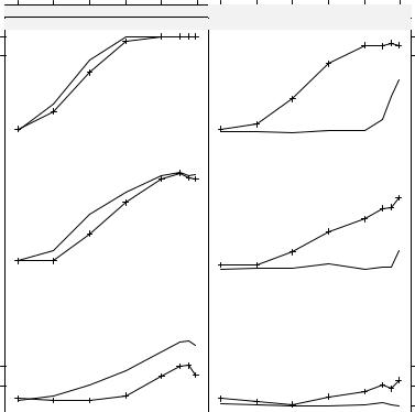
Fig. 7.1. Simulated power curves for dwtest() (solid) and bgtest() (dashed).
2002), specifically aimed at such layouts. It is written in the grid graphics system (Murrell 2005), a system even more flexible than R’s default graphics facilities. grid comes with a multitude of functions and parameters for controlling possibly complex trellis graphics in publication quality. Here, we do not discuss in detail how to use lattice and grid (the interested reader is referred to the associated package documentation) and only demonstrate how to generate Figure 7.1:
R> library("lattice")
R> xyplot(power ~ corr | model + nobs, groups = ~ test, + data = psim, type = "b")
7.2 Bootstrapping a Linear Regression |
189 |
Using xyplot(), a trellis scatterplot is generated for power ~ corr conditional on the combinations of model and nobs. Within each panel, the observations are grouped by test. All data are taken from the simulation results psim, and the plotting type is "b", indicating both (i.e., lines and points). For further control options, see ?xyplot.
In Figure 7.1, rows correspond to varying sample sizes and columns to the underlying model, and each panel shows the power curves as functions of % for both tests. The interpretation is much easier compared to the numerical table: power clearly increases with n and %, and autocorrelation is easier to detect in the trend than in the dynamic model. While the Durbin-Watson test performs slightly better in the trend model for small sample sizes, its power breaks down almost completely in the dynamic model.
7.2 Bootstrapping a Linear Regression
Conventional regression output relies on asymptotic approximations to the distributions of test statistics, which are often not very reliable in small samples or models with substantial nonlinearities. A possible remedy is to employ bootstrap methodology.
In R, a basic recommended package is boot (Canty and Ripley 2008), which provides functions and data sets from Davison and Hinkley (1997). Specifically, the function boot() implements the classical nonparametric bootstrap (sampling with replacement), among other resampling techniques.
Since there is no such thing as “the” bootstrap, the first question is to determine a resampling strategy appropriate for the problem at hand. In econometrics and the social sciences, experimental data are rare, and hence it is appropriate to consider regressors as well as responses as random variables. This suggests employing the pairs bootstrap (i.e., to resample observations), a method that should give reliable standard errors even in the presence of (conditional) heteroskedasticity.
As an illustration, we revisit an example from Chapter 3, the Journals data taken from Stock and Watson (2007). The goal is to compute bootstrap standard errors and confidence intervals by case-based resampling. For ease of reference, we reproduce the basic regression
R> data("Journals")
R> journals <- Journals[, c("subs", "price")]
R> journals$citeprice <- Journals$price/Journals$citations R> jour_lm <- lm(log(subs) ~ log(citeprice), data = journals)
The function boot() takes several arguments, of which data, statistic, and R are required. Here, data is simply the data set and R signifies the number of bootstrap replicates. The second argument, statistic, is a function that returns the statistic to be bootstrapped, where the function itself must take
190 7 Programming Your Own Analysis
the data set and an index vector providing the indices of the observations included in the current bootstrap sample.
This is best understood by considering an example. In our case, the required statistic is given by the convenience function
R> refit <- function(data, i)
+ coef(lm(log(subs) ~ log(citeprice), data = data[i,]))
Now we are ready to call boot():
R> library("boot")
R> set.seed(123)
R> jour_boot <- boot(journals, refit, R = 999)
This yields
R> jour_boot
ORDINARY NONPARAMETRIC BOOTSTRAP
Call:
boot(data = journals, statistic = refit, R = 999)
Bootstrap Statistics : |
|
||
|
original |
bias |
std. error |
t1* |
4.7662 |
-0.0010560 |
0.05545 |
t2* |
-0.5331 |
-0.0001606 |
0.03304 |
A comparison with the standard regression output
R> coeftest(jour_lm)
t test of coefficients:
Estimate Std. Error t value Pr(>|t|)
(Intercept) |
4.7662 |
0.0559 |
85.2 |
<2e-16 |
log(citeprice) |
-0.5331 |
0.0356 |
-15.0 |
<2e-16 |
reveals only minor di erences, suggesting that the conventional version is fairly reliable in this application.
We can also compare bootstrap and conventional confidence intervals. As the bootstrap standard errors were quite similar to the conventional ones, confidence intervals will be expected to be quite similar as well in this example. To save space, we confine ourselves to those of the slope coe cient. The bootstrap provides the interval
R> boot.ci(jour_boot, index = 2, type = "basic")
7.3 Maximizing a Likelihood |
191 |
BOOTSTRAP CONFIDENCE INTERVAL CALCULATIONS
Based on 999 bootstrap replicates
CALL :
boot.ci(boot.out = jour_boot, type = "basic", index = 2)
Intervals : Level Basic
95% (-0.5952, -0.4665 )
Calculations and Intervals on Original Scale
while its classical counterpart is
R> confint(jour_lm, parm = 2)
2.5 % 97.5 % log(citeprice) -0.6033 -0.4628
This underlines that both approaches yield essentially identical results here. Note that boot.ci() provides several further methods for computing bootstrap intervals.
The bootstrap is particularly helpful in situations going beyond leastsquares regression; thus readers are asked to explore bootstrap standard errors in connection with robust regression techniques in an exercise.
Finally, it should be noted that boot contains many further functions for resampling, among them tsboot() for block resampling from time series (for blocks of both fixed and random lengths). Similar functionality is provided by the function tsbootstrap() in the package tseries. In addition, a rather di erent approach, the maximum entropy bootstrap (Vinod 2006), is available in the package meboot.
7.3 Maximizing a Likelihood
Transformations of dependent variables are a popular means to improve the performance of models and are also helpful in the interpretation of results. Zellner and Revankar (1969), in a search for a generalized production function that allows returns to scale to vary with the level of output, introduced (among more general specifications) the generalized Cobb-Douglas form
Yie Yi = eβ1 Kiβ2 Lβi 3 ,
where Y is output, K is capital, and L is labor. From a statistical point of view, this can be seen as a transformation applied to the dependent variable encompassing the level (for = 0, which in this application yields the classical Cobb-Douglas function). Introducing a multiplicative error leads to the logarithmic form
192 7 Programming Your Own Analysis |
|
log Yi + Yi = β1 + β2 log Ki + β3 log Li + "i. |
(7.1) |
However, this model is nonlinear in the parameters, and only for known can it be estimated by OLS. Following Zellner and Ryu (1998) and Greene (2003, Chapter 17), using the Equipment data on transportation equipment manufacturing, we attempt to simultaneously estimate the regression coe - cients and the transformation parameter using maximum likelihood assuming "i N (0, σ2) i.i.d.
The likelihood of the model is |
|
i #, |
|
L = i=1 φ("i/σ) · 1 |
Yi |
||
n |
|
|
|
Y |
+ Y |
|
|
where "i = log Yi + Yi − β1 − β2 log Ki − β3 log Li and φ(·) is the probability density function of the standard normal distribution. Note that @"i/@Yi =
(1 + Yi)/Yi.
This gives the log-likelihood
n |
n |
|
Xi |
X |
|
` = |
{log(1 + Yi) − log Yi} − |
log φ("i/σ). |
=1 |
i=1 |
|
The task is to write a function maximizing this log-likelihood with respect to the parameter vector (β1, β2, β3, , σ2). This decomposes naturally into the following three steps: (1) code the objective function, (2) obtain starting values for an iterative optimization, and (3) optimize the objective function using the starting values.
Step 1: We begin by coding the log-likelihood. However, since the function optim() used below by default performs minimization, we have to slightly modify the natural approach in that we need to minimize the negative of the log-likelihood.
R> data("Equipment", package = "AER")
R> nlogL <- function(par) {
+beta <- par[1:3]
+theta <- par[4]
+sigma2 <- par[5]
+Y <- with(Equipment, valueadded/firms)
+K <- with(Equipment, capital/firms)
+L <- with(Equipment, labor/firms)
+rhs <- beta[1] + beta[2] * log(K) + beta[3] * log(L)
+lhs <- log(Y) + theta * Y
+
+rval <- sum(log(1 + theta * Y) - log(Y) +
+dnorm(lhs, mean = rhs, sd = sqrt(sigma2), log = TRUE))
7.3 Maximizing a Likelihood |
193 |
+return(-rval)
+}
The function nlogL() is a function of a vector parameter par comprising five elements; for convenience, these are labeled as in Equation (7.1). Variables are transformed as needed, after which both sides of Equation (7.1) are set up. These ingredients are then used in the objective function rval, the negative of which is finally returned. Note that R comes with functions for the logarithms of the standard distributions, including the normal density dnorm(..., log
= TRUE).
Step 2: optim() proceeds iteratively, and thus (good) starting values are needed. These can be obtained from fitting the classical Cobb-Douglas form by OLS:
R> fm0 <- lm(log(valueadded/firms) ~ log(capital/firms) +
+log(labor/firms), data = Equipment)
The resulting vector of coe cients, coef(fm0), is now amended by 0, our starting value for , and the mean of the squared residuals from the CobbDouglas fit, the starting value for the disturbance variance:
R> par0 <- as.vector(c(coef(fm0), 0, mean(residuals(fm0)^2)))
Step 3: We are now ready to search for the optimum. The new vector par0 containing all the starting values is used in the call to optim():
R> opt <- optim(par0, nlogL, hessian = TRUE)
By default, optim() uses the Nelder-Mead method, but there are further algorithms available. We set hessian = TRUE in order to obtain standard errors. Parameter estimates, standard errors, and the value of the objective function at the estimates can now be extracted via
R> opt$par
[1] 2.91469 0.34998 1.09232 0.10666 0.04275
R> sqrt(diag(solve(opt$hessian)))[1:4]
[1] 0.36055 0.09671 0.14079 0.05850
R> -opt$value
[1] -8.939
In spite of the small sample, these results suggest that is greater than 0. We add that for practical purposes the solution above needs to be verified;
specifically, several sets of starting values must be examined in order to confirm that the algorithm did not terminate in a local optimum. McCullough (2004) o ers further advice on nonlinear estimation.
Note also that the function presented above is specialized to the data set under investigation. If a reusable function is needed, a proper function