

Kleiber - Applied econometrics in R
.pdf2 |
1 Introduction |
|
|
|
|
[1] "title" |
"publisher" |
"society" |
"price" |
|
[5] "pages" |
"charpp" |
"citations" |
"foundingyear" |
|
[9] "subs" |
"field" |
|
|
reveal that Journals is a data set with 180 observations (the journals) on 10 variables, including the number of library subscriptions (subs), the price, the number of citations, and a qualitative variable indicating whether the journal is published by a society or not.
Here, we are interested in the relation between the demand for economics journals and their price. A suitable measure of the price for scientific journals is the price per citation. A scatterplot (in logarithms), obtained via
R> plot(log(subs) ~ log(price/citations), data = Journals)
and given in Figure 1.1, clearly shows that the number of subscriptions is decreasing with price.
The corresponding linear regression model can be easily fitted by ordinary least squares (OLS) using the function lm() (for linear model) and the same syntax,
R> j_lm <- lm(log(subs) ~ log(price/citations), data = Journals) R> abline(j_lm)
The abline() command adds the least-squares line to the existing scatterplot; see Figure 1.1.
A detailed summary of the fitted model j_lm can be obtained via
R> summary(j_lm)
Call:
lm(formula = log(subs) ~ log(price/citations), data = Journals)
Residuals: |
|
|
|
|
Min |
1Q Median |
3Q |
Max |
|
-2.7248 -0.5361 0.0372 0.4662 1.8481 |
|
|||
Coefficients: |
|
|
|
|
|
Estimate Std. Error t value Pr(>|t|) |
|||
(Intercept) |
4.7662 |
|
0.0559 |
85.2 <2e-16 |
log(price/citations) -0.5331 |
|
0.0356 -15.0 <2e-16 |
||
Residual standard error: 0.75 on 178 degrees of freedom |
||||
Multiple R-squared: 0.557, |
|
Adjusted R-squared: 0.555 |
||
F-statistic: |
224 on 1 and 178 DF, |
p-value: <2e-16 |
||
Specifically, this provides the usual summary of the coe cients (with estimates, standard errors, test statistics, and p values) as well as the associated R2, along with further information. For the journals regression, the estimated

1.1 An Introductory R Session |
3 |
|
7 |
|
6 |
|
5 |
log(subs) |
4 |
|
3 |
|
2 |
|
1 |
|
● |
|
● |
|
|
|
|
|
|
|
|
|
|
|
|
|
|
|
|
|
|
|
|
|
|
|
|
|
|
|
|
|
|
|
|
|
|
|
|
|
|
|
|
|
|
|
|
|
|
|
|
|
|
|
|
|
|
|
|||
|
|
|
|
|
|
|
|
|
|
|
|
|
|
|
|
|
|
|
|
|
|
|
|
|
|
|
|
|
||
|
|
|
● ● |
● |
|
●● |
|
|
● |
|
|
|
|
|
● |
● |
|
|
|
|
|
|
|
|
|
|
|
|
|
|
|
|
|
●● |
|
|
● ●●●●●●● |
|
|
|
|
|
● |
● |
|
|
|
|
|
|
|
|
|
|
|||||||
|
|
|
|
|
|
|
|
●● |
|
|
|
|
|
|
|
|
|
|
|
|
|
|
|
|
|
|
|
|||
|
|
|
|
|
|
|
|
● |
|
|
|
|
|
|
|
|
|
|
|
|
|
|
|
|
|
|
|
|
|
|
|
|
|
● |
|
|
|
|
● |
● ● |
|
|
● |
|
|
● |
|
|
|
|
|
|
|
|
|
|
|
||||
|
|
|
|
|
● |
|
● |
● |
● |
|
● |
|
|
● |
|
|
|
● ● |
|
|
|
|
|
|||||||
|
|
|
|
|
● |
●●● |
● |
● |
|
|
|
|
● |
|
|
|
|
|
||||||||||||
|
|
|
|
|
● |
|
|
● |
● |
|
|
●● |
|
|
|
|
|
|
|
|
|
|
|
|
||||||
|
|
|
|
|
|
● |
|
|
|
● |
● |
|
|
|
|
|
|
|
|
|
|
|
|
|
|
|
||||
|
|
|
|
|
|
|
|
|
|
|
● |
|
|
|
●●●● |
|
● |
|
|
|
|
|
● |
|
|
|||||
|
|
|
|
|
|
|
● |
|
|
|
● |
● |
|
|
|
● |
|
● |
|
|
|
|
|
|
|
|
||||
|
|
|
|
|
|
|
|
|
|
●● |
|
|
● |
|
|
● ● |
|
|
|
|
|
|
|
|||||||
|
|
|
|
|
|
|
|
|
|
|
|
● |
|
|
● |
●● |
● |
|
|
|
|
|
|
|
|
|||||
|
|
|
|
|
|
|
|
|
|
|
|
|
|
|
●●● |
|
|
● |
|
● |
|
|
|
|
|
|
|
|||
|
|
|
|
|
|
|
|
|
|
|
|
● |
●● |
● |
|
● |
|
|
|
|
● |
● |
|
|
|
|
|
|||
|
|
|
|
|
|
|
|
|
|
|
● |
● |
|
|
●● |
|
● |
●●● |
●● |
|
|
|
● |
|
||||||
|
|
|
|
|
|
|
|
|
|
|
|
● |
●● |
● |
●● |
|
|
|
|
|
|
|
|
|||||||
|
|
|
|
|
|
|
|
|
|
|
|
|
|
|
|
●● |
|
● ● |
|
● |
|
|
|
|
|
|||||
|
|
|
|
|
|
|
|
|
|
|
|
|
● ● |
|
● |
● |
● |
|
|
|
|
|
|
● |
||||||
|
|
|
|
|
|
|
|
|
|
|
|
|
● |
● |
|
|
|
|
|
|
|
|||||||||
|
|
|
|
|
|
|
|
|
|
|
|
|
|
|
|
●●● |
●● |
|
● |
● |
●● |
|
●● |
|
|
|||||
|
|
|
|
|
|
|
|
|
|
|
|
|
|
|
|
|
|
● |
● |
|
|
|
●● |
|
●● |
|
|
|||
|
|
|
|
|
|
|
|
|
|
|
|
● |
● |
|
● |
● |
● |
●● |
|
|
|
|
|
|||||||
|
|
|
|
|
|
|
|
|
|
|
|
|
● |
● |
|
● |
●● |
|
|
|
||||||||||
|
|
|
|
|
|
|
|
|
|
|
|
|
|
|
|
|
|
● |
● |
● |
|
|
|
|||||||
|
|
|
|
|
|
|
|
|
|
|
|
|
|
|
|
|
|
|
|
● |
● |
|
●● |
|
|
|
||||
|
|
|
|
|
|
|
|
|
|
|
|
● |
|
|
|
|
|
|
|
|
|
●● |
|
|
|
|||||
|
|
|
|
|
|
|
|
|
|
|
|
|
|
|
|
|
|
● |
|
|
|
|
● |
|
|
● |
|
● |
||
|
|
|
|
|
|
|
|
|
|
|
|
|
|
|
|
|
|
|
|
|
|
|
|
|
||||||
|
|
|
|
|
|
|
|
|
|
|
|
|
|
|
|
|
|
|
|
|
|
|
|
● |
|
|
● |
|||
|
|
|
|
|
|
|
|
|
|
|
|
|
|
|
|
|
|
|
|
|
|
|
● |
|
● |
● |
|
|
|
|
|
|
|
|
|
|
|
|
|
|
|
|
|
|
|
|
|
|
|
|
|
|
|
|
● |
|
|
|
|
|
|
|
|
|
|
|
|
|
|
|
|
|
|
|
|
|
|
|
|
|
|
|
|
|
|
|
|
|
|
|
● |
|
|
|
|
|
|
|
|
|
|
|
|
|
|
|
|
|
|
|
|
|
|
|
|
|
|
|
|
|
|
|
|
|
|
|
|
|
|
|
|
|
|
|
|
|
|
|
|
|
|
|
|
|
|
|
|
|
|
|
|
|
|
|
|
|
|
|
|
|
|
|
|
|
|
|
|
|
|
|
|
|
|
|
|
|
|
|
|
|
|
|
|
|
|
|
|
−4 |
|
|
|
|
−2 |
|
|
|
|
|
|
0 |
|
|
|
|
|
|
|
|
2 |
|
|
|
||||
log(price/citations)
Fig. 1.1. Scatterplot of library subscription by price per citation (both in logs) with least-squares line.
elasticity of the demand with respect to the price per citation is −0.5331, which is significantly di erent from 0 at all conventional levels. The R2 = 0.557 of the model is quite satisfactory for a cross-section regression.
A more detailed analysis with further information on the R commands employed is provided in Chapter 3.
Example 2: Determinants of wages
In the preceding example, we showed how to fit a simple linear regression model to get a flavor of R’s look and feel. The commands for carrying out the analysis often read almost like talking plain English to the system. For performing more complex tasks, the commands become more technical as well—however, the basic ideas remain the same. Hence, all readers should be able to follow the analysis and recognize many of the structures from the previous example even if not every detail of the functions is explained here. Again, the purpose is to provide a motivating example illustrating how easily some more advanced tasks can be performed in R. More details, both on the commands and the data, are provided in subsequent chapters.
The application considered here is the estimation of a wage equation in semi-logarithmic form based on data taken from Berndt (1991). They represent a random subsample of cross-section data originating from the May 1985
4 1 Introduction
Current Population Survey, comprising 533 observations. After loading the data set CPS1985 from the package AER, we first rename it for convenience:
R> data("CPS1985", package = "AER") R> cps <- CPS1985
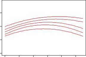
For cps, a wage equation is estimated with log(wage) as the dependent variable and education and experience (both in number of years) as regressors. For experience, a quadratic term is included as well. First, we estimate a multiple linear regression model by OLS (again via lm()). Then, quantile regressions are fitted using the function rq() from the package quantreg. In a sense, quantile regression is a refinement of the standard linear regression model in that it provides a more complete view of the entire conditional distribution (by way of choosing selected quantiles), not just the conditional mean. However, our main reason for selecting this technique is that it illustrates that R’s fitting functions for regression models typically possess virtually identical syntax. In fact, in the case of quantile regression models, all we need to specify in addition to the already familiar formula and data arguments is tau, the set of quantiles that are to be modeled; in our case, this argument will be set to 0.2, 0.35, 0.5, 0.65, 0.8.
After loading the quantreg package, both models can thus be fitted as easily as
R> library("quantreg")
R> cps_lm <- lm(log(wage) ~ experience + I(experience^2) +
+education, data = cps)
R> cps_rq <- rq(log(wage) ~ experience + I(experience^2) +
+education, data = cps, tau = seq(0.2, 0.8, by = 0.15))
These fitted models could now be assessed numerically, typically with a summary() as the starting point, and we will do so in a more detailed analysis in Chapter 4. Here, we focus on graphical assessment of both models, in particular concerning the relationship between wages and years of experience. Therefore, we compute predictions from both models for a new data set cps2, where education is held constant at its mean and experience varies over the range of the original variable:
R> cps2 <- data.frame(education = mean(cps$education),
+experience = min(cps$experience):max(cps$experience)) R> cps2 <- cbind(cps2, predict(cps_lm, newdata = cps2,
+interval = "prediction"))
R> cps2 <- cbind(cps2,
+predict(cps_rq, newdata = cps2, type = ""))
For both models, predictions are computed using the respective predict() methods and binding the results as new columns to cps2. First, we visualize the results of the quantile regressions in a scatterplot of log(wage) against experience, adding the regression lines for all quantiles (at the mean level of education):
1.1 An Introductory R Session |
5 |
|
|
● |
|
|
|
|
|
|
|
|
|
|
|
|
|
|
|
|
|
|
|
|
|
|
|
|
|
|
|
|
|
|
|
|
|
●● |
|
|
|
|
|
|
|
●● |
|
● |
● ●● |
|
● ● |
● |
|
|
● ● |
|
|
|
|
||||||
|
3 |
|
● |
|
|
● |
|
● ●● |
● |
|
|
●● |
|
|
|
● |
|
|
|||||||||||||
|
|
|
|
|
● |
● |
|
●● |
|
|
|
|
● |
|
|
●● |
|
|
|
|
|
|
|
|
|
||||||
|
|
|
|
● |
|
● |
|
● |
|
|
|
|
|
|
|
|
|
|
● |
|
|
● ● |
|
|
|
|
|
|
|||
|
|
|
|
|
|
|
|
●●● |
|
●●● |
|
|
|
|
|
|
|
● |
|
|
|
|
|
|
|||||||
|
|
|
|
● |
|
● |
|
|
●●● |
● |
● |
● ● ● |
|
|
|
● |
|
|
●● ● |
|
|
|
|||||||||
|
|
|
|
|
|
|
|
●●● |
● |
● |
|
|
|
|
|
|
|
|
● |
|
|
||||||||||
|
|
|
|
|
|
|
●●●● |
|
●●● |
|
|
|
|
● |
|
|
|
●● |
|
|
● |
|
|
● |
|
|
|||||
|
|
|
|
|
|
|
|
●●● |
●● ● |
|
|
|
|
|
|
● |
|
|
|
|
|
|
|
||||||||
|
|
|
|
●● |
|
●●●●●● |
● |
● |
● |
● |
|
●● |
|
● |
|
|
|
● |
|
|
|
|
|
● |
|
|
|
||||
|
|
|
● |
● |
● |
|
● |
● |
●●● |
●● |
● |
|
|
● |
●● |
● |
|
● |
● |
|
● |
|
|
●●● |
|
● |
|
||||
log(wage) |
|
● |
|
● |
● |
|
● |
●● |
|
|
● |
● |
|
●● |
|
●● |
|
|
|
|
|
|
|||||||||
|
|
● |
|
●● |
●●●●● |
|
|
● |
●● |
|
|
● |
|
●● |
●● |
|
●●● |
|
|
● |
|
● |
|||||||||
|
|
|
● |
|
|
|
|
●● |
●● |
|
|
●● |
●● |
|
|
|
● |
● |
|
|
|||||||||||
|
|
●●● |
●●●●● |
●●● |
● |
●● |
● |
●● |
● |
|
●● |
● |
|
● |
|
|
|
|
● |
||||||||||||
|
|
|
|
● |
|
● |
● |
|
|
|
|
|
|
● |
|
|
|
|
●● |
|
|
||||||||||
|
|
|
|
|
|
●● |
|
● |
●● |
● |
|
●●●● ● |
|
|
|
|
|
● |
|
|
|
|
|||||||||
2 |
●●● ●●●●●● |
|
|
●●● |
●● |
|
|
|
|
|
|
|
|
|
|
|
|
||||||||||||||
|
● |
● |
|
●●● |
|
● |
●● |
● |
|
|
● ● |
|
● |
|
|
● ●●● |
|
● |
● ● |
● |
|
|
● |
||||||||
|
|
|
● |
|
|
|
|
|
|
|
|
● |
|||||||||||||||||||
●● |
●● |
● |
●●●● |
|
● |
● |
|
|
|
●● |
|
● |
● |
|
|
● |
|
● |
|
||||||||||||
●● |
● |
|
|
|
● ● |
|
● |
|
|
|
|
● |
|
|
● |
|
|
|
|
|
|
● |
|||||||||
● |
● |
|
|
●●● |
|
● |
|
● |
|
● |
|
|
|
● |
|
|
● |
● ● |
|
|
|
|
● |
|
|
||||||
|
● |
●●●● |
|
●● |
●●● |
|
|
|
● |
|
|
|
● |
|
|
|
|
|
|
● |
|
||||||||||
● |
● |
● |
|
|
● |
|
|
● ●● |
|
|
|
● |
|
● |
|
|
●● |
|
|
|
|
||||||||||
●●●●● |
|
● |
●●●● |
● |
● |
|
|
● ● |
|
|
|
|
|
|
● |
|
● |
|
|||||||||||||
●● |
|
|
● |
● |
● |
|
●● |
● |
|
●● |
|
|
|
● |
|
|
|
● |
|
●● |
|
|
|
● |
|
||||||
● |
●●● |
|
● |
|
|
●●● |
|
|
|
● |
|
|
● |
|
|
|
|
|
|
|
|||||||||||
|
|
● |
● |
● |
|
|
|
● |
|
● |
|
|
● |
|
● |
● |
|
|
|
|
|
●● |
|
|
|
|
● |
||||
|
|
● |
|
● |
●●●● |
● |
● |
|
|
|
|
|
|
|
|
|
|
|
|
|
● |
|
|
|
|||||||
|
|
|
|
● |
|
● |
● |
●● |
|
|
|
|
● |
|
|
|
|
|
|
|
|
|
●● |
|
|
|
|||||
|
|
● |
|
|
● |
|
● |
|
|
|
● |
|
|
|
|
● |
|
|
|
|
●●● |
|
● |
|
|
|
|
●● |
|||
|
|
● |
●● |
|
|
●●●● |
|
● |
|
|
|
|
|
|
|
|
● |
● |
|
|
|
|
|
|
|
● |
|
|
● |
||
|
1 |
● |
|
|
|
|
|
|
|
|
|
|
|
|
|
|
|
|
|
|
|
|
|
|
|
|
● |
|
|
|
|
|
|
|
|
|
|
|
|
|
|
|
|
|
|
|
|
|
|
|
|
|
|
|
|
|
|
|
|
|
|
||
|
|
|
|
|
|
|
|
|
|
|
|
|
|
|
|
|
|
|
|
|
|
|
|
|
|
|
|
|
|
|
|
|
|
● |
|
● |
|
|
|
|
|
|
|
|
|
|
|
|
|
|
|
|
|
|
|
|
|
|
|
|
|
|
|
|
|
|
|
|
|
|
|
|
|
|
|
|
|
|
|
|
|
|
|
|
|
|
|
|
|
|
|
|
|
|
|
|
0 |
|
|
|
|
|
|
|
|
|
|
|
|
|
|
● |
|
|
|
|
|
|
|
|
|
|
|
|
|
|
|
|
|
0 |
|
|
|
|
10 |
|
|
|
|
20 |
|
|
|
|
|
30 |
|
|
|
|
40 |
|
|
|
50 |
||||
|
|
|
|
|
|
|
|
|
|
|
|
|
|
|
experience |
|
|
|
|
|
|
|
|
|
|||||||
Fig. 1.2. Scatterplot of log-wage versus experience, with quantile regression fits for varying quantiles.
R> plot(log(wage) ~ experience, data = cps)
R> for(i in 6:10) lines(cps2[,i] ~ experience,
+data = cps2, col = "red")
To keep the code compact, all regression lines are added in a for() loop. The resulting plot is displayed in Figure 1.2, showing that wages are highest for individuals with around 30 years of experience. The curvature of the regression lines is more marked at lower quartiles, whereas the relationship is much flatter for higher quantiles. This can also be seen in Figure 1.3, obtained via
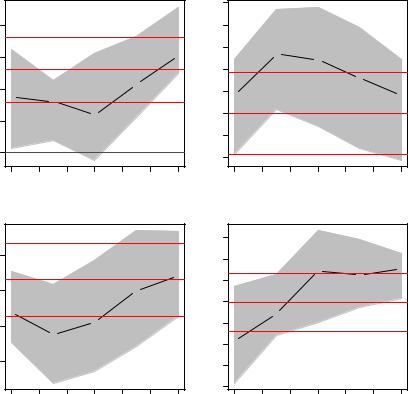
R> plot(summary(cps_rq))
which depicts the changes in the regression coe cients over varying quantiles along with the least-squares estimates (both together with 90% confidence intervals). This shows that both experience coe cients are eventually decreasing in absolute size (note that the coe cient on the quadratic term is negative) with increasing quantile and that consequently the curve is flatter for higher quantiles. The intercept also increases, while the influence of education does not vary as much with the quantile level.
Although the size of the sample in this illustration is still quite modest by current standards, with 533 observations many observations are hidden due to overplotting in scatterplots such as Figure 1.2. To avoid this problem, and to further illustrate some of R’s graphics facilities, kernel density estimates will
6 1 Introduction
|
|
(Intercept) |
|
|
||
0.8 |
|
|
|
|
|
0.055 |
0.6 |
|
|
|
|
|
● |
|
|
|
|
|
0.045 |
|
0.4 |
|
|
|
|
● |
|
|
|
|
|
|
|
|
● |
|
|
|
|
|
|
|
|
● |
|
|
|
0.035 |
0.2 |
|
|
● |
|
|
|
|
|
|
|
|
||
0.0 |
|
|
|
|
|
0.025 |
0.2 |
0.3 |
0.4 |
0.5 |
0.6 |
0.7 |
0.8 |
|
|
I(experience^2) |
|
|
||
−4e−04 |
|
|
|
|
|
0.11 |
04 |
|
|
|
|
|
● |
|
|
|
|
|
|
|
−6e− |
|
|
|
|
● |
|
|
|
|
|
|
0.09 |
|
● |
|
|
|
|
|
|
−04 |
|
|
● |
|
|
|
|
|
|
|
|
|
|
03 −8e |
|
● |
|
|
|
0.07 |
|
|
|
|
|
||
−1e− |
|
|
|
|
|
|
|
|
|
|
|
|
0.05 |
0.2 |
0.3 |
0.4 |
0.5 |
0.6 |
0.7 |
0.8 |
|
|
experience |
|
|
||
|
|
● |
|
|
|
|
|
|
|
● |
|
|
|
|
|
|
|
|
● |
|
● |
|
|
|
|
|
● |
0.2 |
0.3 |
0.4 |
0.5 |
0.6 |
0.7 |
0.8 |
|
|
|
education |
|
|
|
|
|
|
|
|
|
● |
|
|
|
● |
|
|
|
|
|
|
|
|
● |
|
|
|
● |
|
|
|
|
● |
|
|
|
|
|
|
0.2 |
0.3 |
0.4 |
0.5 |
0.6 |
0.7 |
0.8 |
Fig. 1.3. Coe cients of quantile regression for varying quantiles, with confidence bands (gray) and least-squares estimate (red).
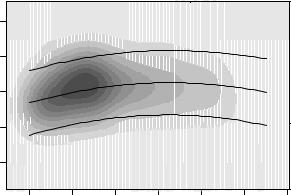
be used: highversus low-density regions in the bivariate distribution can be identified by a bivariate kernel density estimate and brought out graphically in a so-called heatmap. In R, the bivariate kernel density estimate is provided by bkde2D() in the package KernSmooth:
R> library("KernSmooth")
R> cps_bkde <- bkde2D(cbind(cps$experience, log(cps$wage)),
+bandwidth = c(3.5, 0.5), gridsize = c(200, 200))
As bkde2D() does not have a formula interface (in contrast to lm() or rq()), we extract the relevant columns from the cps data set and select suitable bandwidths and grid sizes. The resulting 200 200 matrix of density estimates
1.1 An Introductory R Session |
7 |
|
4 |
|
|
|
|
|
|
|
3 |
|
|
|
|
|
|
log(wage) |
2 |
|
|
|
|
|
|
|
1 |
|
|
|
|
|
|
|
0 |
|
|
|
|
|
|
|
0 |
10 |
20 |
30 |
40 |
50 |
60 |
|
|
|
|
experience |
|
|
|
Fig. 1.4. Bivariate kernel density heatmap of log-wage by experience, with leastsquares fit and prediction interval.
can be visualized in a heatmap using gray levels coding the density values. R provides image() (or contour()) to produce such displays, which can be applied to cps_bkde as follows.
R> image(cps_bkde$x1, cps_bkde$x2, cps_bkde$fhat,
+col = rev(gray.colors(10, gamma = 1)),
+xlab = "experience", ylab = "log(wage)") R> box()
R> lines(fit ~ experience, data = cps2)
R> lines(lwr ~ experience, data = cps2, lty = 2) R> lines(upr ~ experience, data = cps2, lty = 2)
After drawing the heatmap itself, we add the regression line for the linear model fit along with prediction intervals (see Figure 1.4). Compared with the scatterplot in Figure 1.2, this brings out more clearly the empirical relationship between log(wage) and experience.
This concludes our introductory R session. More details on the data sets, models, and R functions are provided in the following chapters.
8 1 Introduction
1.2 Getting Started
The R system for statistical computing and graphics (R Development Core Team 2008b, http://www.R-project.org/) is an open-source software project, released under the terms of the GNU General Public License (GPL), Version 2. (Readers unfamiliar with open-source software may want to visit http://www.gnu.org/.) Its source code as well as several binary versions can be obtained, at no cost, from the Comprehensive R Archive Network (CRAN;
see http://CRAN.R-project.org/mirrors.html to find its nearest mirror site). Binary versions are provided for 32-bit versions of Microsoft Windows, various flavors of Linux (including Debian, Red Hat, SUSE, and Ubuntu) and Mac OS X.
Installation
Installation of binary versions is fairly straightforward: just go to CRAN, pick the version corresponding to your operating system, and follow the instructions provided in the corresponding readme file. For Microsoft Windows, this amounts to downloading and running the setup executable (.exe file), which takes the user through a standard setup manager. For Mac OS X, separate disk image .dmg files are available for the base system as well as for a GUI developed for this platform. For various Linux flavors, there are prepackaged binaries (as .rpm or .deb files) that can be installed with the usual packaging tools on the respective platforms. Additionally, versions of R are also distributed in many of the standard Linux repositories, although these are not necessarily as quickly updated to new R versions as CRAN is.
For every system, in particular those for which a binary package does not exist, there is of course also the option to compile R from the source. On some platforms, notably Microsoft Windows, this can be a bit cumbersome because the required compilers are typically not part of a standard installation. On other platforms, such as Unix or Linux, this often just amounts to the usual configure/make/install steps. See R Development Core Team (2008d) for detailed information on installation and administration of R.
Packages
As will be discussed in greater detail below, base R is extended by means of packages, some of which are part of the default installation. Packages are stored in one or more libraries (i.e., collections of packages) on the system and can be loaded using the command library(). Typing library() without any arguments returns a list of all currently installed packages in all libraries. In the R world, some of these are referred to as “base” packages (contained in the R sources); others are “recommended” packages (included in every binary distribution). A large number of further packages, known as “contributed” packages (currently more than 1,400), are available from the CRAN servers
(see http://CRAN.R-project.org/web/packages/), and some of these will
1.3 Working with R |
9 |
be required as we proceed. Notably, the package accompanying this book, named AER, is needed. On a computer connected to the Internet, its installation is as simple as typing
R> install.packages("AER")
at the prompt. This installation process works on all operating systems; in addition, Windows users may install packages by using the “Install packages from CRAN” and Mac users by using the “Package installer” menu option and then choosing the packages to be installed from a list. Depending on the installation, in particular on the settings of the library paths, install.packages() by default might try to install a package in a directory where the user has no writing permission. In such a case, one needs to specify the lib argument or set the library paths appropriately (see R Development Core Team 2008d, and ?library for more information). Incidentally, installing AER will download several further packages on which AER depends. It is not uncommon for packages to depend on other packages; if this is the case, the package “knows” about it and ensures that all the functions it depends upon will become available during the installation process.
To use functions or data sets from a package, the package must be loaded. The command is, for our package AER,
R> library("AER")
From now on, we assume that AER is always loaded. It will be necessary to install and load further packages in later chapters, and it will always be indicated what they are.
In view of the rapidly increasing number of contributed packages, it has proven to be helpful to maintain a number of “CRAN task views” that provide an overview of packages for certain tasks. Current task views include econometrics, finance, social sciences, and Bayesian statistics. See
http://CRAN.R-project.org/web/views/ for further details.
1.3 Working with R
There is an important di erence in philosophy between R and most other econometrics packages. With many packages, an analysis will lead to a large amount of output containing information on estimation, model diagnostics, specification tests, etc. In R, an analysis is normally broken down into a series of steps. Intermediate results are stored in objects, with minimal output at each step (often none). Instead, the objects are further manipulated to obtain the information required.
In fact, the fundamental design principle underlying R (and S) is “everything is an object”. Hence, not only vectors and matrices are objects that can be passed to and returned by functions, but also functions themselves, and even function calls. This enables computations on the language and can considerably facilitate programming tasks, as we will illustrate in Chapter 7.
10 1 Introduction
Handling objects
To see what objects are currently defined, the function objects() (or equivalently ls()) can be used. By default, it lists all objects in the global environment (i.e., the user’s workspace):
R> objects()
[1] |
"CPS1985" |
"Journals" |
"cps" |
"cps2" |
"cps_bkde" |
[6] |
"cps_lm" |
"cps_rq" |
"i" |
"j_lm" |
|
which returns a character vector of length 9 telling us that there are currently nine objects, resulting from the introductory session.
However, this cannot be the complete list of available objects, given that some objects must already exist prior to the execution of any commands, among them the function objects() that we just called. The reason is that the search list, which can be queried by
R> search()
[1] |
".GlobalEnv" |
"package:KernSmooth" |
[3] |
"package:quantreg" |
"package:SparseM" |
[5] |
"package:AER" |
"package:survival" |
[7] |
"package:splines" |
"package:strucchange" |
[9] |
"package:sandwich" |
"package:lmtest" |
[11] |
"package:zoo" |
"package:car" |
[13] |
"package:stats" |
"package:graphics" |
[15] |
"package:grDevices" |
"package:utils" |
[17] |
"package:datasets" |
"package:methods" |
[19] |
"Autoloads" |
"package:base" |
comprises not only the global environment ".GlobalEnv" (always at the first position) but also several attached packages, including the base package at its end. Calling objects("package:base") will show the names of more than a thousand objects defined in base, including the function objects() itself.
Objects can easily be created by assigning a value to a name using the assignment operator <-. For illustration, we create a vector x in which the number 2 is stored:
R> x <- 2
R> objects()
[1] |
"CPS1985" |
"Journals" |
"cps" |
"cps2" |
"cps_bkde" |
[6] |
"cps_lm" |
"cps_rq" |
"i" |
"j_lm" |
"x" |
x is now available in our global environment and can be removed using the function remove() (or equivalently rm()):
R> remove(x)
R> objects()
|
|
1.3 Working with R |
11 |
|
[1] "CPS1985" |
"Journals" "cps" |
"cps2" |
"cps_bkde" |
|
[6] "cps_lm" |
"cps_rq" "i" |
"j_lm" |
|
|
Calling functions
If the name of an object is typed at the prompt, it will be printed. For a function, say foo, this means that the corresponding R source code is printed (try, for example, objects), whereas if it is called with parentheses, as in foo(), it is a function call. If there are no arguments to the function, or all arguments have defaults (as is the case with objects()), then foo() is a valid function call. Therefore, a pair of parentheses following the object name is employed throughout this book to signal that the object discussed is a function.
Functions often have more than one argument (in fact, there is no limit to the number of arguments to R functions). A function call may use the arguments in any order, provided the name of the argument is given. If names of arguments are not given, R assumes they appear in the order of the function definition. If an argument has a default, it may be left out in a function call. For example, the function log() has two arguments, x and base: the first, x, can be a scalar (actually also a vector), the logarithm of which is to be taken; the second, base, is the base with respect to which logarithms are computed.
Thus, the following four calls are all equivalent:
R> log(16, 2)
R> log(x = 16, 2)
R> log(16, base = 2)
R> log(base = 2, x = 16)
Classes and generic functions
Every object has a class that can be queried using class(). Classes include “data.frame” (a list or array with a certain structure, the preferred format in which data should be held), “lm” for linear-model objects (returned when fitting a linear regression model by ordinary least squares; see Section 1.1 above), and “matrix” (which is what the name suggests). For each class, certain methods to so-called generic functions are available; typical examples include summary() and plot(). The result of these functions depends on the class of the object: when provided with a numerical vector, summary() returns basic summaries of an empirical distribution, such as the mean and the median; for a vector of categorical data, it returns a frequency table; and in the case of a linear-model object, the result is the standard regression output. Similarly, plot() returns pairs of scatterplots when provided with a data frame and returns basic diagnostic plots for a linear-model object.