

Kleiber - Applied econometrics in R
.pdf6.2 Classical Model-Based Analysis |
163 |
Standardized Residuals
−3 −2 −1 0 1 2
1955 |
1960 |
1965 |
1970 |
Time
ACF of Residuals
ACF −0.2 0.2 0.6 1.0
0 |
1 |
2 |
3 |
4 |
Lag
|
1.0 |
|
0.8 |
p value |
0.4 0.6 |
|
0.2 |
|
0.0 |
|
|
|
|
p values for Ljung−Box statistic |
|
|
|
|
|
|
|
|||||
|
|
|
|
|
|
|
|
|
|
|
|
|
|
|
||
|
|
|
|
● |
● |
|
|
|
|
|
|
|
||||
|
|
|
|
|
|
|
|
|
|
|
|
|
|
|||
|
● |
● |
|
|
|
|
|
|
● |
● |
||||||
|
|
|
|
|
|
|
|
|
|
|
|
|
|
|||
|
|
|
|
|
|
|
|
|
|
● |
|
|
|
|
||
|
● |
|
|
|
|
|
● |
|
|
|
|
|
|
|
||
|
|
|
|
● |
|
|
|
|
|
|
|
|||||
|
|
|
|
|
|
|
|
|
|
|
|
|
|
|
|
|
|
|
|
|
|
|
|
|
|
|
|
|
|
|
|
|
|
|
|
|
|
|
|
|
|
|
|
|
|
|
|
|
|
|
|
2 |
4 |
6 |
8 |
|
10 |
||||||||||
|
|
|
|
|
|
|
lag |
|
|
|
|
|
|
|
||
Fig. 6.7. Diagnostics for SARIMA(0, 1, 1)(0, 1, 1)4 model.
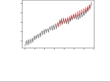
Figure 6.8 shows that the general trend is captured reasonably well. However, the model systematically overpredicts for certain parts of the sample in the 1980s.
We conclude by adding that there exist, apart from generic functions such as coef(), logLik(), predict(), print(), and vcov(), which also work on objects of class “Arima” (the class of objects returned by arima()), several further convenience functions for exploring ARMA models and their representations. These are listed in Table 6.2.
164 6 Time Series
|
11.0 |
|
|
|
|
|
|
|
log(UKNonDurables) |
10.4 10.6 10.8 |
|
|
|
|
|
|
|
|
10.2 |
|
|
|
|
|
|
|
|
1955 |
1960 |
1965 |
1970 |
1975 |
1980 |
1985 |
1990 |
|
|
|
|
Time |
|
|
|
|
|
Fig. 6.8. |
Predictions from SARIMA(0, 1, 1)(0, 1, 1)4 model. |
||||||
Table 6.2. Convenience functions for ARMA models.
Function |
Package |
Description |
|
|
|
acf2AR() |
stats |
Computes an AR process exactly fitting a given autocor- |
|
|
relation function. |
|
|
|
arima.sim() |
stats |
Simulation of ARIMA models. |
|
|
|
ARMAacf() |
stats |
Computes theoretical (P)ACF for a given ARMA model. |
|
|
|
ARMAtoMA() |
stats |
Computes MA(1) representation for a given ARMA |
|
|
model. |
|
|
|
6.3 Stationarity, Unit Roots, and Cointegration
Many time series in macroeconomics and finance are nonstationary, the precise form of the nonstationarity having caused a hot debate some 25 years ago. Nelson and Plosser (1982) argued that macroeconomic time series often are more appropriately described by unit-root nonstationarity than by deterministic time trends. We refer to Hamilton (1994) for an overview of the methodology. The Nelson and Plosser data (or rather an extended version ending in 1988) are available in R in the package tseries (Trapletti 2008), and we shall use them for an exercise at the end of this chapter.
6.3 Stationarity, Unit Roots, and Cointegration |
165 |
|
7000 |
black |
|
|
|
|
|
|
|
|
|
|
|
|
|
white |
|
|
|
|
PepperPrice |
3000 5000 |
|
|
|
|
|
|
1000 |
|
|
|
|
|
|
|
1975 |
1980 |
1985 |
1990 |
1995 |
|
|
|
|
Time |
|
|
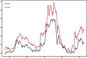
Fig. 6.9. Time series of average monthly European spot prices for black and white pepper (fair average quality) in US dollars per ton.
To illustrate the main methods, we employ a di erent data set, PepperPrice, containing a bivariate time series of average monthly European spot prices for black and white pepper in US dollars per ton. The data are taken from Franses (1998) and are part of the AER package accompanying this book. Figure 6.9 plots both series, and for obvious reasons they are rather similar:
R> data("PepperPrice")
R> plot(PepperPrice, plot.type = "single", col = 1:2) R> legend("topleft", c("black", "white"), bty = "n",
+col = 1:2, lty = rep(1,2))
We begin with an investigation of the time series properties of the individual series, specifically determining their order of integration. There are two ways to proceed: one can either test the null hypothesis of di erence stationarity against stationarity (the approach of the classical unit-root tests) or reverse the roles of the alternatives and use a stationarity test such as the KPSS test (Kwiatkowski, Phillips, Schmidt, and Shin 1992).
Unit-root tests
The test most widely used by practitioners, the augmented Dickey-Fuller (ADF) test (Dickey and Fuller 1981), is available in the function adf.test()
166 6 Time Series
from the package tseries (Trapletti 2008). This function implements the t test of H0 : % = 0 in the regression
|
k |
|
|
yt = + δt + %yt−1 + |
Xj |
yt−j + "t. |
(6.3) |
φj |
|||
|
=1 |
|
|
The number of lags k defaults to b(n−1)1/3c but may be changed by the user. For the series corresponding to the price of white pepper, the test yields
R> library("tseries")
R> adf.test(log(PepperPrice[, "white"]))
Augmented Dickey-Fuller Test
data: log(PepperPrice[, "white"])
Dickey-Fuller = -1.744, Lag order = 6, p-value = 0.6838 alternative hypothesis: stationary
while, for the series of first di erences, we obtain
R> adf.test(diff(log(PepperPrice[, "white"])))
Augmented Dickey-Fuller Test
data: diff(log(PepperPrice[, "white"])) Dickey-Fuller = -5.336, Lag order = 6, p-value = 0.01 alternative hypothesis: stationary
Warning message:
In adf.test(diff(log(PepperPrice[, "white"]))) : p-value smaller than printed p-value
Note that a warning is issued because the p value is only interpolated from a few tabulated critical values, and hence no p values outside the interval [0.01, 0.1] can be provided.
Alternatively, the Phillips-Perron test (Phillips and Perron 1988) with its nonparametric correction for autocorrelation (essentially employing a HAC estimate of the long-run variance in a Dickey-Fuller-type test (6.3) instead of parametric decorrelation) can be used. It is available in the function pp.test() from the package tseries (there also exists a function PP.test() in base R, but it has fewer options). Using the default options to the PhillipsPerron t test in the equation with a time trend, we obtain
R> pp.test(log(PepperPrice[, "white"]), type = "Z(t_alpha)")
Phillips-Perron Unit Root Test
data: log(PepperPrice[, "white"])
6.3 Stationarity, Unit Roots, and Cointegration |
167 |
Dickey-Fuller Z(t_alpha) = -1.6439, Truncation lag parameter = 5, p-value = 0.726
alternative hypothesis: stationary
Thus, all tests suggest that the null hypothesis of a unit root cannot be rejected here. Alternative implementations of the preceding methods with somewhat di erent interfaces are available in the package urca (Pfa 2006). That package also o ers a function ur.ers() implementing the test of Elliott, Rothenberg, and Stock (1996), which utilizes GLS detrending.
Stationarity tests
Kwiatkowski et al. (1992) proceed by testing for the presence of a random walk component rt in the regression
yt = dt + rt + "t,
where dt denotes a deterministic component and "t is a stationary—more precisely, I(0)—error process. This test is also available in the function kpss.test() in the package tseries. The deterministic component is either a constant or a linear time trend, the former being the default. Setting the argument null = "Trend" yields the second version. Here, we obtain
R> kpss.test(log(PepperPrice[, "white"]))
KPSS Test for Level Stationarity
data: log(PepperPrice[, "white"])
KPSS Level = 0.9129, Truncation lag parameter = 3, p-value = 0.01
Hence the KPSS test also points to nonstationarity of the pepper price series. (Again, a warning is issued, as the p value is interpolated from the four critical values provided by Kwiatkowski et al. 1992, it is suppressed here.)
Readers may want to check that the series pertaining to black pepper yields similar results when tested for unit roots or stationarity.
Cointegration
The very nature of the two pepper series already suggests that they possess common features. Having evidence for nonstationarity, it is of interest to test for a common nonstationary component by means of a cointegration test.
A simple method to test for cointegration is the two-step method proposed by Engle and Granger (1987). It regresses one series on the other and performs a unit root test on the residuals. This test, often named after Phillips and Ouliaris (1990), who provided the asymptotic theory, is available in the function po.test() from the package tseries. Specifically, po.test() performs a
168 6 Time Series
Phillips-Perron test using an auxiliary regression without a constant and linear trend and the Newey-West estimator for the required long-run variance. A regression of the price for black pepper on that for white pepper yields
R> po.test(log(PepperPrice))
Phillips-Ouliaris Cointegration Test
data: log(PepperPrice)
Phillips-Ouliaris demeaned = -24.0987, Truncation lag parameter = 2, p-value = 0.02404
suggesting that both series are cointegrated. (Recall that the first series pertains to black pepper. The function proceeds by regressing the first series on the remaining ones.) A test utilizing the reverse regression is as easy as po.test(log(PepperPrice[,2:1])). However, the problem with this approach is that it treats both series in an asymmetric fashion, while the concept of cointegration demands that the treatment be symmetric.
The standard tests proceeding in a symmetric manner stem from Johansen’s full-information maximum likelihood approach (Johansen 1991). For a pth-order cointegrated vector autoregressive (VAR) model, the error correction form is (omitting deterministic components)
|
p−1 |
|
yt = yt−1 + |
Xj |
yt−j + "t. |
+j |
||
|
=1 |
|
The relevant tests are available in the function ca.jo() from the package urca. The basic version considers the eigenvalues of the matrix in the preceding equation. We again refer to Hamilton (1994) for the methodological background.
Here, we employ the trace statistic—the maximum eigenvalue, or “lambdamax”, test is available as well—in an equation amended by a constant term (specified by ecdet = "const"), yielding
R> library("urca")
R> pepper_jo <- ca.jo(log(PepperPrice), ecdet = "const", + type = "trace")
R> summary(pepper_jo)
######################
# Johansen-Procedure #
######################
Test type: trace statistic , without linear trend and constant in cointegration
Eigenvalues (lambda):
6.4 Time Series Regression and Structural Change |
169 |
[1] 4.93195e-02 1.35081e-02 1.38778e-17
Values of teststatistic and critical values of test:
test 10pct 5pct 1pct r <= 1 | 3.66 7.52 9.24 12.97 r = 0 | 17.26 17.85 19.96 24.60
Eigenvectors, normalised to first column: (These are the cointegration relations)
black.l2 white.l2 constant black.l2 1.000000 1.00000 1.00000 white.l2 -0.889231 -5.09942 2.28091 constant -0.556994 33.02742 -20.03244
Weights W:
(This is the loading matrix)
black.l2 white.l2 constant black.d -0.0747230 0.00245321 3.86752e-17 white.d 0.0201561 0.00353701 4.03196e-18
The null hypothesis of no cointegration is rejected; hence the Johansen test confirms the results from the initial two-step approach.
6.4 Time Series Regression and Structural Change
More on fitting dynamic regression models
As already discussed in Chapter 3, there are various ways of fitting dynamic linear regression models by OLS in R. Here, we present two approaches in more detail: (1) setting up lagged and di erenced regressors “by hand” and calling lm(); (2) using the convenience interface dynlm() from the package dynlm (Zeileis 2008). We illustrate both approaches using a model for the UKDriverDeaths series: the log-casualties are regressed on their lags 1 and 12, essentially corresponding to the multiplicative SARIMA(1, 0, 0)(1, 0, 0)12 model
yt = β1 + β2 yt−1 + β3 yt−12 + "t, t = 13, . . . , 192.
For using lm() directly, we set up a multivariate time series containing the original log-casualties along with two further variables holding the lagged observations. The lagged variables are created with lag(). Note that its second argument, the number of lags, must be negative to shift back the observations. For “ts” series, this just amounts to changing the "tsp" attribute (leaving the
170 6 Time Series
observations unchanged), whereas for “zoo” series k observations have to be omitted for computation of the kth lag. For creating unions or intersections of several “ts” series, ts.union() and ts.intersect() can be used, respectively. For “zoo” series, both operations are provided by the merge() method. Here, we use ts.intersect() to combine the original and lagged series, assuring that leading and trailing NAs are omitted before the model fitting. The final call to lm() works just as in the preceding sections because lm() does not need to know that the underlying observations are from a single time series.
R> dd <- log(UKDriverDeaths)
R> dd_dat <- ts.intersect(dd, dd1 = lag(dd, k = -1),
+dd12 = lag(dd, k = -12))
R> lm(dd ~ dd1 + dd12, data = dd_dat)
Call:
lm(formula = dd ~ dd1 + dd12, data = dd_dat)
Coefficients: |
|
|
(Intercept) |
dd1 |
dd12 |
0.421 |
0.431 |
0.511 |
The disadvantage is that lm() cannot preserve time series properties of the data unless further e ort is made (specifically, setting dframe = TRUE in ts.intersect() and na.action = NULL in lm(); see ?lm for details). Even then, various nuisances remain, such as using di erent na.actions, print output formatting, or subset selection.
The function dynlm() addresses these issues. It provides an extended model language in which di erences and lags can be directly specified via d() and L() (using the opposite sign of lag() for the second argument), respectively. Thus
R> library("dynlm")
R> dynlm(dd ~ L(dd) + L(dd, 12))
Time series regression with "ts" data:
Start = 1970(1), End = 1984(12)
Call:
dynlm(formula = dd ~ L(dd) + L(dd, 12))
Coefficients: |
|
|
(Intercept) |
L(dd) |
L(dd, 12) |
0.421 |
0.431 |
0.511 |
yields the same results as above, but the object returned is a “dynlm” object inheriting from “lm” and provides additional information on the underlying time stamps. The same model could be written somewhat more concisely as

6.4 Time Series Regression and Structural Change |
171 |
dd ~ L(dd, c(1, 12)). Currently, the disadvantage of dynlm() compared with lm() is that it cannot be reused as easily with other functions. However, as dynlm is still under development, this is likely to improve in future versions.
Structural change tests
As we have seen in previous sections, the structure in the series of logcasualties did not remain the same throughout the full sample period: there seemed to be a decrease in the mean number of casualties after the policy change in seatbelt legislation. Translated into a parametric time series model, this means that the parameters of the model are not stable throughout the sample period but change over time.
The package strucchange (Zeileis, Leisch, Hornik, and Kleiber 2002) implements a large collection of tests for structural change or parameter instability that can be broadly placed in two classes: (1) fluctuation tests and (2) tests based on F statistics. Fluctuation tests try to assess the structural stability by capturing fluctuation in cumulative or moving sums (CUSUMs or MOSUMs) of residuals (OLS or recursive), model scores (i.e., empirical estimating functions), or parameter estimates (from recursively growing or from rolling data windows). The idea is that, under the null hypothesis of parameter stability, the resulting “fluctuation processes” are governed by a functional central limit theorem and only exhibit limited fluctuation, whereas under the alternative of structural change, the fluctuation is generally increased. Thus, there is evidence for structural change if an appropriately chosen empirical fluctuation process crosses a boundary that the corresponding limiting process crosses only with probability . In strucchange, empirical fluctuation processes can be fitted via efp(), returning an object of class “efp” that has a plot() method for performing the corresponding test graphically and an sctest() method (for structural change test) for a traditional significance test with test statistic and p value.
Here, we use an OLS-based CUSUM test (Ploberger and Kramer¨ 1992) to assess the stability of the SARIMA-type model for the UK driver deaths data fitted at the beginning of this section. The OLS-based CUSUM process is
simply the scaled cumulative sum process of the OLS residuals ˆ = − > ˆ;
that is,
"t yt xt β
1 |
|
bnsc |
|
|
|
efp(s) = |
σˆp |
|
Xt |
"ˆt, |
0 s 1. |
|
|
||||
n |
=1 |
||||
It can be computed with the function efp() by supplying formula and data (as for lm()) and setting in addition type = "OLS-CUSUM":
R> dd_ocus <- efp(dd ~ dd1 + dd12, data = dd_dat,
+type = "OLS-CUSUM")
The associated structural change test, by default considering the maximum absolute deviation of the empirical fluctuation process from zero and given by
172 6 Time Series
R> sctest(dd_ocus)
OLS-based CUSUM test
data: dd_ocus
S0 = 1.4866, p-value = 0.02407
is significant at the default 5% level, signaling that the model parameters are not stable throughout the entire sample period. The plot in the left panel of Figure 6.10 results from
R> plot(dd_ocus)
and yields some further insights. In addition to the excessive fluctuation (conveyed by the boundary crossing), it can be seen from the peak in the process that an abrupt change seems to have taken place in about 1973(10), matching the timing of the first oil crisis. A smaller second peak in the process, associated with the change of seatbelt legislation in 1983(1), is also visible.
Tests based on F statistics, the second class of tests in strucchange, are designed to have good power for single-shift alternatives (of unknown timing). The basic idea is to compute an F statistic (or Chow statistic) for each conceivable breakpoint in a certain interval and reject the null hypothesis of structural stability if any of these statistics (or some other functional such as the mean) exceeds a certain critical value (Andrews 1993; Andrews and Ploberger 1994). Processes of F statistics can be fitted with Fstats(), employing an interface similar to efp(). The resulting “Fstats” objects can again be assessed by the corresponding sctest() method or graphically by the plot() method. The code chunk
R> dd_fs <- Fstats(dd ~ dd1 + dd12, data = dd_dat, from = 0.1) R> plot(dd_fs)
R> sctest(dd_fs)
supF test
data: dd_fs
sup.F = 19.3331, p-value = 0.006721
uses the supF test of Andrews (1993) for the SARIMA-type model with a trimming of 10%; i.e., an F statistic is computed for each potential breakpoint between 1971(6) and 1983(6), omitting the leading and trailing 10% of observations. The resulting process of F statistics is shown in the right panel of Figure 6.10, revealing two clear peaks in 1973(10) and 1983(1). Both the boundary crossing and the tiny p value show that there is significant departure from the null hypothesis of structural stability. The two peaks in the F process also demonstrate that although designed for single-shift alternatives, the supF test has power against multiple-shift alternatives. In this case, it brings out the two breaks even more clearly than the OLS-based CUSUM test.