Kleiber - Applied econometrics in R

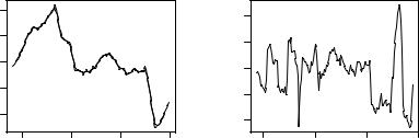
Fig. 6.1. Quarterly time series of consumption of non-durables in the United Kingdom (left) and monthly number of car drivers killed or seriously injured in the United Kingdom (right, with filtered version).

reconstructing all time stamps). Both are major nuisances when working with irregular series (e.g., with many financial time series). Consequently, various implementations for irregular time series have emerged in contributed R packages, the most flexible of which is “zoo”, provided by the zoo1 package (Zeileis and Grothendieck 2005). It can have time stamps of arbitrary type and is designed to be as similar as possible to “ts”. Specifically, the series are essentially also numeric vectors or matrices but with an "index" attribute containing the full vector of indexes (or time stamps) rather than only the "tsp" attribute with start/end/frequency. Therefore, “zoo” series can be seen as a generalization of “ts” series. Most methods that work for “ts” objects also work for “zoo” objects, some have extended functionality, and some new ones are provided. Regular series can be coerced back and forth between the classes without loss of information using the functions as.zoo() and as.ts(). Hence, it does not make much di erence which of these two classes is used for annual, quarterly, or monthly data—whereas “zoo” is much more convenient for daily data (e.g., coupled with an index of class “Date”) or intraday data (e.g., with “POSIXct” or “chron” time stamps). See Zeileis and Grothendieck (2005) for further details on “zoo” series and Grothendieck and Petzoldt (2004) for more on date/time classes in R.

Throughout this book, we mainly rely on the “ts” class; only in very few illustrations where additional flexibility is required do we switch to “zoo”.

1zoo stands for Z’s ordered observations, named after the author who started the development of the package.

154 6 Time Series

(Linear) filtering

One of the most basic tools for transforming time series (e.g., for eliminating seasonality) is linear filtering (see Brockwell and Davis 1991, 1996). An important class of linear filters are finite moving averages, transformations that replace the raw data yt by a weighted sum

yˆt = Xs ajyt+j, t = r + 1, . . . , n − s.

j=−r

If r equals s, the filter is called symmetric. In R, the function filter() permits the use of fairly general filters; its argument filter takes a vector containing the coe cients aj. Apart from moving averages (default, see above), filter() can also apply recursive linear filters, another important class of filters.

As an example, we consider the monthly time series UKDriverDeaths containing the well-known data from Harvey and Durbin (1986) on car drivers killed or seriously injured in the United Kingdom from 1969(1) through 1984(12). These are also known as the “seatbelt data”, as they were used by Harvey and Durbin (1986) for evaluating the e ectiveness of compulsory wearing of seatbelts introduced on 1983-01-31. The following code loads and plots the series along with a filtered version utilizing the simple symmetric moving average of length 13 with coe cients (1/24, 1/12, . . . , 1/12, 1/24)>.

R> data("UKDriverDeaths") R> plot(UKDriverDeaths)

R> lines(filter(UKDriverDeaths, c(1/2, rep(1, 11), 1/2)/12),

+col = 2)

The resulting plot is depicted in the right panel of Figure 6.1, illustrating that the filter eliminates seasonality. Other classical filters, such as the Henderson or Spencer filters (Brockwell and Davis 1991), can be applied analogously.

Another function that can be used for evaluating linear and nonlinear functions on moving data windows is rollapply() (for rolling apply). This can be used for computing running means via rollapply(UKDriverDeaths, 12, mean), yielding a result similar to that for the symmetric filter above, or running standard deviations

R> plot(rollapply(UKDriverDeaths, 12, sd))

shown in the right panel of Figure 6.2, revealing increased variation around the time of the policy intervention.

As mentioned above, filter() also provides autoregressive (recursive) filtering. This can be exploited for simple simulations; e.g., from AR(1) models. The code

R> set.seed(1234)

R> x <- filter(rnorm(100), 0.9, method = "recursive")

Fig. 6.2. UK driver deaths: trends from two season-trend decompositions (left) and running standard deviations (right).

generates 100 observations from an AR(1) process with parameter 0.9 and standard normal innovations. A more elaborate tool for simulating from general ARIMA models is provided by arima.sim().

Decomposition

Filtering with moving averages can also be used for an additive or multiplicative decomposition into seasonal, trend, and irregular components. The classical approach to this task, implemented in the function decompose(), is to take a simple symmetric filter as illustrated above for extracting the trend and derive the seasonal component by averaging the trend-adjusted observations from corresponding periods. A more sophisticated approach that also accommodates time-varying seasonal components is seasonal decomposition via loess smoothing (Cleveland, Cleveland, McRae, and Terpenning 1990). It is available in the function stl() and iteratively finds the seasonal and trend components by loess smoothing of the observations in moving data windows of a certain size. Both methods are easily applied in R using (in keeping with the original publication, we employ logarithms)

R> dd_dec <- decompose(log(UKDriverDeaths))

R> dd_stl <- stl(log(UKDriverDeaths), s.window = 13)

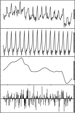
where the resulting objects dd_dec and dd_stl hold the trend, seasonal, and irregular components in slightly di erent formats (a list for the “decomposed.ts” and a multivariate time series for the “stl” object). Both classes have plotting methods drawing time series plots of the components with a common time axis. The result of plot(dd_stl) is provided in Figure 6.3, and the result of plot(dd_dec) looks rather similar. (The bars

156 6 Time Series

Fig. 6.3. Season-trend decomposition by loess smoothing.

at the right side of Figure 6.3 are of equal heights in user coordinates to ease interpretation.) A graphical comparison of the fitted trend components, obtained via

R> plot(dd_dec$trend, ylab = "trend")

R> lines(dd_stl$time.series[,"trend"], lty = 2, lwd = 2)

and given in Figure 6.2 (left panel), reveals that both methods provide qualitatively similar results, with stl() yielding a smoother curve. Analogously, the seasonal components dd_stl$time.series[,"seasonal"] and dd_dec$seasonal could be extracted and compared. We note that stl() has artificially smoothed over the structural break due to the introduction of

Holt−Winters filtering

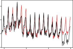
Fig. 6.4. Predictions from Holt-Winters exponential smoothing.

seatbelts, inducing some rather large values in the remainder series. We shall come back to this example in Section 6.4 using di erent methods.

Exponential smoothing

Another application of linear filtering techniques are classical forecasting methods of the exponential smoothing type, such as simple or double exponential smoothing, employing recursively reweighted lagged observations for predicting future data. A general framework for this is Holt-Winters smoothing (see Meyer 2002, for a brief introduction in R), which comprises these and related exponential smoothing techniques as special cases. The function HoltWinters() implements the general methodology—by default computing a Holt-Winters filter with an additive seasonal component, determining the smoothing parameters by minimizing the squared prediction error on the observed data. To illustrate its use, we separate the UKDriverDeaths series into a historical sample up to 1982(12) (i.e., before the change in legislation) and use Holt-Winters filtering to predict the observations for 1983 and 1984.

R> dd_past <- window(UKDriverDeaths, end = c(1982, 12)) R> dd_hw <- HoltWinters(dd_past)

R> dd_pred <- predict(dd_hw, n.ahead = 24)

Figure 6.4 compares Holt-Winters predictions with the actually observed series after the policy intervention via

158 6 Time Series

R> plot(dd_hw, dd_pred, ylim = range(UKDriverDeaths)) R> lines(UKDriverDeaths)

showing that the number of road casualties clearly dropped after the introduction of mandatory wearing of seatbelts.

We conclude by noting that a more sophisticated function for exponential smoothing algorithms, named ets(), is available in the package forecast (Hyndman and Khandakar 2008).

6.2 Classical Model-Based Analysis

The classical approach to parametric modeling and forecasting is to employ an autoregressive integrated moving average (ARIMA) model for capturing the dependence structure in a time series (Brockwell and Davis 1991; Box and Jenkins 1970; Hamilton 1994). To fix the notation, ARIMA(p, d, q) models are defined by the equation

where the autoregressive (AR) part is given by the pth-order polynomial φ(L) = 1 − φ1L − . . . − φpLp in the lag operator L, the moving average (MA) part is given by the qth-order polynomial (L) = 1+ 1L+. . .+ qLq, and d is the order of di erencing. (Note the sign convention for the MA polynomial.)

For ease of reference, Table 6.1 provides a partial list of time series fitting functions (with StructTS() being discussed in Section 6.5).

Fig. 6.5. (Partial) autocorrelation function.

Table 6.1. Time series fitting functions in R.

Before fitting an ARIMA model to a series, it is helpful to first take an exploratory look at the empirical ACF and PACF. In R, these are available in the functions acf() and pacf(), respectively. For the artificial AR(1) process x from the previous section, they are computed and plotted by

R> acf(x)

R> pacf(x)

and shown in Figure 6.5. Here, the maximum number of lags defaults to 10 log10(n), but it can be changed by the argument lag.max. Plotting can be suppressed by setting plot = FALSE. This is useful when the (P)ACF is needed for further computations.

The empirical ACF for series x decays only slowly, while the PACF exceeds the individual confidence limits only for lag 1, reflecting clearly how the series was generated. Next we try to recover the true structure by fitting an autoregression to x via the function ar():

R> ar(x)

Call: ar(x = x)

Coefficients:

1

0.928

160 6 Time Series

Order selected 1 sigma^2 estimated as 1.29

This agrees rather well with the true autocorrelation of 0.9. By default, ar() fits AR models up to lag p = 10 log10(n) and selects the minimum AIC model. This is usually a good starting point for model selection, even though the default estimator is the Yule-Walker estimator, which is considered a preliminary estimator. ML is also available in addition to OLS and Burg estimation; see ?ar for further details.

For a real-world example, we return to the UKNonDurables series, aiming at establishing a model for the (log-transformed) observations up to 1970(4) for predicting the remaining series.

R> nd <- window(log(UKNonDurables), end = c(1970, 4))

The corresponding time series plot (see Figure 6.1) suggests rather clearly that di erencing is appropriate; hence the first row of Figure 6.6 depicts the empirical ACF and PACF of the di erenced series. As both exhibit a strong seasonal pattern (already visible in the original series), the second row of Figure 6.6 also shows the empirical ACF and PACF after double di erencing (at the seasonal lag 4 and at lag 1) as generated by

R> acf(diff(nd), ylim = c(-1, 1))

R> pacf(diff(nd), ylim = c(-1, 1))

R> acf(diff(diff(nd, 4)), ylim = c(-1, 1))

R> pacf(diff(diff(nd, 4)), ylim = c(-1, 1))

For this series, a model more general than a simple AR model is needed: arima() fits general ARIMA models, including seasonal ARIMA (SARIMA) models and models containing further regressors (utilizing the argument xreg), either via ML or minimization of the conditional sum of squares (CSS). The default is to use CSS to obtain starting values and then ML for refinement. As the model space is much more complex than in the AR(p) case, where only the order p has to be chosen, base R does not o er an automatic model selection method for general ARIMA models based on information criteria. Therefore, we use the preliminary results from the exploratory analysis above and R’s general tools to set up a model search for an appropriate SARIMA(p, d, q)(P, D, Q)4 model,

which amends the standard ARIMA model (6.1) by additional polynomials operating on the seasonal frequency.

The graphical analysis clearly suggests double di erencing of the original series (d = 1, D = 1), some AR and MA e ects (we allow p = 0, 1, 2 and q = 0, 1, 2), and low-order seasonal AR and MA parts (we use P = 0, 1 and Q = 0, 1), giving a total of 36 parameter combinations to consider. Of course, higher values for p, q, P , and Q could also be assessed. We refrain from doing so

Fig. 6.6. (Partial) autocorrelation functions for UK non-durables data.

to save computation time in this example—however, we encourage readers to pursue this issue for higher-order models as well. We also note that the package forecast (Hyndman and Khandakar 2008) contains a function auto.arima() that performs a search over a user-defined set of models, just as we do here manually. To choose from the 36 possible models, we set up all parameter combinations via expand.grid(), fit each of the associated SARIMA models using arima() in a for() loop, and store the resulting BIC extracted from the model (obtained via AIC() upon setting k = log(length(nd))).

R> nd_pars <- expand.grid(ar = 0:2, diff = 1, ma = 0:2, + sar = 0:1, sdiff = 1, sma = 0:1)

R> nd_aic <- rep(0, nrow(nd_pars))

R> for(i in seq(along = nd_aic)) nd_aic[i] <- AIC(arima(nd,

162 6 Time Series

+unlist(nd_pars[i, 1:3]), unlist(nd_pars[i, 4:6])),

+k = log(length(nd)))

R> nd_pars[which.min(nd_aic),]

ar diff ma sar sdiff sma

These computations reveal that a SARIMA(0, 1, 1)(0, 1, 1)4 model is best in terms of BIC, conforming well with the exploratory analysis. This model is also famously known as the airline model due to its application to a series of airline passengers in the classical text by Box and Jenkins (1970). It is refitted to nd via

R> nd_arima <- arima(nd, order = c(0,1,1), seasonal = c(0,1,1)) R> nd_arima

Call:

arima(x = nd, order = c(0, 1, 1), seasonal = c(0, 1, 1))

Coefficients:

ma1 sma1 -0.353 -0.583 s.e. 0.143 0.138

sigma^2 estimated as 9.65e-05: log likelihood = 188.14, aic = -370.27

showing that both moving average coe cients are negative and significant. To assess whether this model appropriately captures the dependence structure of the series, tsdiag() produces several diagnostic plots

R> tsdiag(nd_arima)

shown in Figure 6.7. In the first panel, the standardized residuals are plotted. They do not exhibit any obvious pattern. Their empirical ACF in the second panel shows no (individually) significant autocorrelation at lags > 1. Finally, the p values for the Ljung-Box statistic in the third panel all clearly exceed 5% for all orders, indicating that there is no significant departure from white noise for the residuals.

As there are no obvious deficiencies in our model, it is now used for predicting the remaining 18 years in the sample:

R> nd_pred <- predict(nd_arima, n.ahead = 18 * 4)

The object nd_pred contains the predictions along with their associated standard errors and can be compared graphically with the observed series via

R> plot(log(UKNonDurables))

R> lines(nd_pred$pred, col = 2)