Kleiber - Applied econometrics in R

Table 5.1. Selected GLM families and their canonical (default) links.

Similarly, for binary data, the Bernoulli distribution (a special case of the binomial distribution) is suitable, and here we have

which shows that the logit transform log{p/(1 − p)}, the quantile function of the logistic distribution, corresponds to the canonical link for the binary regression model. A widely used non-canonical link for this model is the quantile function of the standard normal distribution, yielding the probit link.

Table 5.1 provides a summary of the most important examples of generalized linear models. A more complete list may be found in standard references on GLMs such as McCullagh and Nelder (1989).

In view of the built-in distributional assumption, it is natural to estimate a GLM by the method of maximum likelihood. For the GLM with a normally distributed response and the identity link, the MLE reduces to the leastsquares estimator and is therefore available in closed form. In general, there is no closed-form expression for the MLE; instead it must be determined using numerical methods. For GLMs, the standard algorithm is called iterative weighted least squares (IWLS). It is an implementation of the familiar Fisher scoring algorithm adapted for GLMs.

These analogies with the classical linear model suggest that a fitting function for GLMs could look almost like the fitting function for the linear model, lm(). In R, this is indeed the case. The fitting function for GLMs is called glm(), and its syntax closely resembles the syntax of lm(). Of course, there are extra arguments for selecting the response distribution and the link function, but apart from this, the familiar arguments such as formula, data, weights, and subset are all available. In addition, all the extractor functions from Table 3.1 have methods for objects of class “glm”, the class of objects returned by glm().

5.2 Binary Dependent Variables

Regression problems with binary dependent variables are quite common in microeconometrics, usually under the names of logit and probit regressions. The model is

124 5 Models of Microeconometrics

E(yi|xi) = pi = F (x>i β), i = 1, . . . , n,

where F equals the standard normal CDF in the probit case and the logistic CDF in the logit case. As noted above, fitting logit or probit models proceeds using the function glm() with the appropriate family argument (including a specification of the link function). For binary responses (i.e., Bernoulli outcomes), the family is binomial, and the link is specified either as link = "logit" or link = "probit", the former being the default. (A look at ?glm reveals that there are further link functions available, but these are not commonly used in econometrics.)

To provide a typical example, we again turn to labor economics, considering female labor force participation for a sample of 872 women from Switzerland. The data were originally analyzed by Gerfin (1996) and are also used by Davidson and MacKinnon (2004). The dependent variable is participation, which we regress on all further variables plus age squared; i.e., on income, education, age, age^2, numbers of younger and older children (youngkids and oldkids), and on the factor foreign, which indicates citizenship. Following Gerfin (1996), we begin with a probit regression:

R> data("SwissLabor")

R> swiss_probit <- glm(participation ~ . + I(age^2),

+ data = SwissLabor, family = binomial(link = "probit")) R> summary(swiss_probit)

Call:

glm(formula = participation ~ . + I(age^2),

family = binomial(link = "probit"), data = SwissLabor)

Deviance Residuals:

Coefficients:

Estimate Std. Error z value Pr(>|z|)

(Dispersion parameter for binomial family taken to be 1)

Null deviance: 1203.2 on 871 degrees of freedom

Residual deviance: 1017.2 on 864 degrees of freedom AIC: 1033

Number of Fisher Scoring iterations: 4

This shows that the summary of a “glm” object closely resembles the summary of an “lm” object: there are a brief summary of the residuals and a table providing coe cients, standard errors, etc., and this is followed by some further summary measures. Among the di erences is the column labeled z value. It provides the familiar t statistic (the estimate divided by its standard error), but since it does not follow an exact t distribution here, even under ideal conditions, it is commonly referred to its asymptotic approximation, the normal distribution. Hence, the p value comes from the standard normal distribution here. For the current model, all variables except education are highly significant. The dispersion parameter (denoted φ in (5.1)) is taken to be 1 because the binomial distribution is a one-parameter exponential family. The deviance resembles the familiar residual sum of squares. Finally, the number of Fisher scoring iterations is provided, which indicates how quickly the IWLS algorithm terminates.

Visualization

Traditional scatterplots are of limited use in connection with binary dependent variables. When plotting participation versus a continuous regressor such as age using

R> plot(participation ~ age, data = SwissLabor, ylevels = 2:1)

R by default provides a so-called spinogram, which is similar to the spine plot introduced in Section 2.8. It first groups the regressor age into intervals, just as in a histogram, and then produces a spine plot for the resulting proportions of participation within the age groups. Note that the horizontal axis is distorted because the width of each age interval is proportional to the corresponding number of observations. By setting ylevels = 2:1, the order of participation levels is reversed, highlighting participation (rather than non-participation). Figure 5.1 shows the resulting plot for the regressors education and age, indicating an approximately quadratic relationship between participation and age and slight nonlinearities between

participation and education.

E ects

e ects in a probit regression model vary with the regressors. Researchers often state average marginal e ects when reporting results from a binary

oldkids I(age^2) -0.058617 -0.117384

and

R> av["foreign"] * coef(swiss_probit)[-7]

This indicates that all e ects are smaller in absolute size for the foreign women. Furthermore, methods for visualizing e ects in linear and generalized linear

models are available in the package e ects (Fox 2003).

Goodness of fit and prediction

In contrast to the linear regression model, there is no commonly accepted version of R2 for generalized linear models, not even for the special case of binary dependent variables.

R2 measures for nonlinear models are often called pseudo-R2s. If we define

( ˆ) as the log-likelihood for the fitted model and (¯) as the log-likelihood

` β ` y

for the model containing only a constant term, we can use a ratio of log-

likelihoods,

( ˆ) R2 = 1 − ``(¯βy) ,

often called McFadden’s pseudo-R2. This is easily made available in R by computing the null model, and then extracting the logLik() values for the two models

R> swiss_probit0 <- update(swiss_probit, formula = . ~ 1) R> 1 - as.vector(logLik(swiss_probit)/logLik(swiss_probit0))

[1] 0.1546

yields a rather modest pseudo-R2 for the model fitted to the SwissLabor data. In the first line of the code chunk above, the update() call reevaluates the original call using the formula corresponding to the null model. In the second line, as.vector() strips o all additional attributes returned by logLik() (namely the "class" and "df" attributes).

A further way of assessing the fit of a binary regression model is to compare the categories of the observed responses with their fitted values. This requires prediction for GLMs. The generic function predict() also has a method for objects of class “glm”. However, for GLMs, things are slightly more involved than for linear models in that there are several types of predictions. Specifically, the predict() method for “glm” objects has a type argument allowing

128 5 Models of Microeconometrics

types "link", "response", and "terms". The default "link" is on the scale of the linear predictors, and "response" is on the scale of the mean of the response variable. For a binary regression model, the default predictions are thus of probabilities on the logit or probit scales, while type = "response" yields the predicted probabilities themselves. (In addition, the "terms" option returns a matrix giving the fitted values of each term in the model formula on the linear-predictor scale.)

In order to obtain the predicted class, we round the predicted probabilities and tabulate the result against the actual values of participation in a confusion matrix,

R> table(true = SwissLabor$participation,

+pred = round(fitted(swiss_probit)))

pred true 0 1

no 337 134 yes 146 255

corresponding to 67.89% correctly classified and 32.11% misclassified observations in the observed sample.

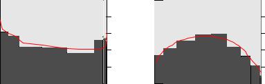
However, this evaluation of the model uses the arbitrarily chosen cuto 0.5 for the predicted probabilities. To avoid choosing a particular cuto , the performance can be evaluated for every conceivable cuto ; e.g., using (as above) the“accuracy”of the model, the proportion of correctly classified observations, as the performance measure. The left panel of Figure 5.2 indicates that the best accuracy is achieved for a cuto slightly below 0.5.

Alternatively, the receiver operating characteristic (ROC) curve can be used: for every cuto c 2 [0, 1], the associated true positive rate (TPR(c), in our case the number of women participating in the labor force that are also classified as participating compared with the total number of women participating) is plotted against the false positive rate (FPR(c), in our case the number of women not participating in the labor force that are classified as participating compared with the total number of women not participating). Thus, ROC = {(FPR(c), TPR(c)) | c 2 [0, 1]}, and this curve is displayed in the right panel of Figure 5.2. For a sensible predictive model, the ROC curve should be at least above the diagonal (which corresponds to random guessing). The closer the curve is to the upper left corner (FPR = 0, TPR = 1), the better the model performs.

In R, visualizations of these (and many other performance measures) can be created using the ROCR package (Sing, Sander, Beerenwinkel, and Lengauer 2005). In the first step, the observations and predictions are captured in an object created by prediction(). Subsequently, various performances can be computed and plotted:

R> library("ROCR")

R> pred <- prediction(fitted(swiss_probit),

Fig. 5.2. Accuracy and ROC curve for labor force probit regression.

+ SwissLabor$participation) R> plot(performance(pred, "acc"))

R> plot(performance(pred, "tpr", "fpr")) R> abline(0, 1, lty = 2)

Figure 5.2 indicates that the fit is reasonable but also that there is room for improvement. We will reconsider this problem at the end of this chapter using semiparametric techniques.

Residuals and diagnostics

For residual-based diagnostics, a residuals() method for “glm” objects is available. It provides various types of residuals, the most prominent of which are deviance and Pearson residuals. The former are defined as (signed) contributions to the overall deviance of the model and are computed by default in R. The latter are the raw residuals yi −µˆi scaled by the standard error (often called standardized residuals in econometrics) and are available by setting type = "pearson". Other types of residuals useful in certain situations and readily available via the residuals() method are working, raw (or response), and partial residuals. The associated sums of squares can be inspected using

R> deviance(swiss_probit)

[1] 1017

R> sum(residuals(swiss_probit, type = "deviance")^2)

[1] 1017

R> sum(residuals(swiss_probit, type = "pearson")^2)

130 5 Models of Microeconometrics

[1] 866.5

and an analysis of deviance is performed by the anova() method for “glm” objects. Other standard tests for nested model comparisons, such as waldtest(),

linear.hypothesis(), and coeftest(), are available as well.

We also note that sandwich estimates of the covariance matrix are available in the usual manner, and thus

R> coeftest(swiss_probit, vcov = sandwich)

would give the usual regression output with robustified standard errors and t statistics. However, the binary case di ers from the linear regression model in that it is not possible to misspecify the variance while correctly specifying the regression equation. Instead, both are either correctly specified or not. Thus, users must be aware that, in the case where conventional and sandwich standard errors are very di erent, there are likely to be problems with the regression itself and not just with the variances of the estimates. Therefore, we do not recommend general use of sandwich estimates in the binary regression case (see also Freedman 2006, for further discussion). Sandwich estimates are much more useful and less controversial in Poisson regressions, as discussed in the following section.

(Quasi-)complete separation

To conclude this section, we briefly discuss an issue that occasionally arises with probit or logit regressions. For illustration, we consider a textbook example inspired by Stokes (2004). The goal is to study the deterrent e ect of capital punishment in the United States of America in 1950 utilizing the MurderRates data taken from Maddala (2001). Maddala uses these data to illustrate probit and logit models, apparently without noticing that there is a problem.

Running a logit regression of an indicator of the incidence of executions (executions) during 1946–1950 on the median time served of convicted murderers released in 1951 (time in months), the median family income in 1949 (income), the labor force participation rate (in percent) in 1950 (lfp), the proportion of the population that was non-Caucasian in 1950 (noncauc), and a factor indicating region (southern) yields, using the defaults of the estimation process,

R> data("MurderRates")

R> murder_logit <- glm(I(executions > 0) ~ time + income +

+noncauc + lfp + southern, data = MurderRates,

+family = binomial)

Warning message:

fitted probabilities numerically 0 or 1 occurred in: glm.fit(x = X, y = Y, weights = weights, start = start,

Thus, calling glm() results in a warning message according to which some fitted probabilities are numerically identical to zero or one. Also, the standard error of southern is suspiciously large:

R> coeftest(murder_logit)

z test of coefficients:

Estimate Std. Error z value Pr(>|z|)

Clearly, this model deserves a closer look. The warning suggests that numerical problems were encountered, so it is advisable to modify the default settings of the IWLS algorithm in order to determine the source of the phenomenon. The relevant argument to glm() is control, which takes a list consisting of the entries epsilon, the convergence tolerance epsilon, maxit, the maximum number of IWLS iterations, and trace, the latter indicating if intermediate output is required for each iteration. Simultaneously decreasing the epsilon and increasing the maximum number of iterations yields

R> murder_logit2 <- glm(I(executions > 0) ~ time + income +

+noncauc + lfp + southern, data = MurderRates,

+family = binomial, control = list(epsilon = 1e-15,

+maxit = 50, trace = FALSE))

Warning message:

fitted probabilities numerically 0 or 1 occurred in: glm.fit(x = X, y = Y, weights = weights, start = start,

Interestingly, the warning does not go away and the coe cient on southern has doubled, accompanied by a 6,000-fold increase of the corresponding standard error:

R> coeftest(murder_logit2)

z test of coefficients:

Estimate Std. Error z value Pr(>|z|)

132 5 Models of Microeconometrics

The explanation of this phenomenon is somewhat technical: although the likelihood of the logit model is known to be globally concave and bounded from above, this does not imply that an interior maximum exists. This is precisely the problem we encountered here, and it depends on the settings of the function call when and where the algorithm terminates. Termination does not mean that a maximum was found, just that it was not possible to increase the objective function beyond the tolerance epsilon supplied. Specifically, we have here a situation where the maximum likelihood estimator does not exist. Instead, there exists a β0 such that

If this is the case, the data are said to exhibit quasi-complete separation (the case of strict inequalities being called complete separation). Although the e ect is not uncommon with small data sets, it is rarely discussed in textbooks; Davidson and MacKinnon (2004) is an exception.

For the problem at hand, the change in the coe cient on southern already indicates that this variable alone is responsible for the e ect. A tabulation reveals

R> table(I(MurderRates$executions > 0), MurderRates$southern)

no yes FALSE 9 0 TRUE 20 15

In short, all of the 15 southern states, plus 20 of the remaining ones, executed convicted murderers during the period in question; thus the variable southern alone contains a lot of information on the dependent variable.

In practical terms, complete or quasi-complete separation is not necessarily a nuisance. After all, we are able to perfectly distinguish the zeros from the ones. However, many practitioners find it counterintuitive, if not disturbing, that the nonexistence of the MLE might be beneficial in some situations. Note also that inspection of the individual t statistics in coeftest(murder_logit) suggests excluding southern. As a result, the warning would have gone away, but the predictions would have been worse. The message is to carefully study such warnings in regressions with a binary dependent variable, with huge standard errors often pointing to the source of the problem.

5.3 Regression Models for Count Data

In this section, we consider a number of regression models for count data. A convenient reference on the methodological background is Cameron and Trivedi (1998). For illustration, we use the RecreationDemand data previously analyzed by Ozuna and Gomez (1995) and Gurmu and Trivedi (1996),