Genomics- The Science and Technology Behind the Human Genome Project. Charles R. Cantor, Cassandra L / genomics1-10 / 3

BASIC REQUIREMENTS FOR SELECTIVITY AND SENSITIVITY

65

BOX 3.1

BINOMIAL

STATISTICS

Binomial

statistics

describe

the

probable outcome of events like coin

flipping,

events that depend on a

single random variable. While a normal coin has a

50%

chance of heads or tails

with each flip, we will consider here the more general

case

of

a

weighted

coin

with

two

possible

outcomes

with

probabilities

p

(heads)

and

q

(tails). Since there are no other possible outcomes

p

q

1. If N

successive flips

are executed, and the outcome is a particular string, such as

hhhhttthhh,

the

chance

of this particular outcome is

p n q N n ,

where

n

is the number

of times heads was ob-

served. Note that all strings with the same numbers of heads and tails will have the

same a priori probability, since in binomial statistics each event does not affect the

probability of subsequent events. Later in this book we will deal with cases where

this extremely simple model does not hold. If we care only about the chance of an

outcome

with

n

heads

and

N

n

tails,

without regard

to

sequence,

the

number of

such

events

is

N

!/(n !)(N n )!, and so the fraction of

times

this

outcome

will

be

seen is (

p n q N n )N !/(n !)(N n )!

A simple binomial model can also be used to estimate the frequency of

occur-

rence

of

particular

DNA

base sequences. Here there are four possible outcomes

(not quite as complex as dice throwing where six possible outcomes occur). For a

particular

string

with

n A A’s,

n C

C’s,

n G

G’s and

n T

T’s, and

a base

composition

of

n T .

X

A

,

X

C

,

X

G

,

and

X

T

the

chance occurrence

of

that

string

is

X

n A X

n C X

n G X

The

A

C

G

T

number of possible strings with a particular base composition is

N

!/(n A

!n C !n G !n T !),

and by combining this with the previous term, the probability of a string with a par-

ticular base composition can easily be computed. Incidentally, the number of possi-

ble strings

of

length

N

is

4 N

, while

the

number

of different

base

compositions

of

this length is (

N

3)!/(N !3!).

The

same

statistical

models can

be used to make estimates that two people

will

share the same DNA sequences. Such estimates are very useful in DNA-based identity

testing. Here we consider just the simple case of two allele polymorphisms. In a par-

ticular place in the genome, suppose that a fraction of all individuals have one base,

f1 ,

while the remainder have another,

f2. The chance that two individuals share

the

same

allele is

f

1

2 f

2

2

g

2. If

a set

of

M

two-allele

polymorphisms

(

i, j, k, . . .)

is consid-

ered

simultaneously,

the

chance

that

two

individuals

are

identical

for

all

of

them is

g

2i g j2g k2. .

. .

By

choosing

M

sufficiently

large,

we

can

clearly

make

the

overall

chance too low to occur,

unless the individuals in question are one and the

same.

However, two caveats apply to this

reasoning. First, related individuals will

show

a

much higher degree of similarity than predicted by this model. Monozygotic twins, in

principle, should share an identical set of alleles at the germ-line level. Second, the

proper allele frequencies to use will depend on the racial, ethnic, and other genetic

characteristics of the individuals in question. Thus it may not always be easy to select

appropriate values. These difficulties notwithstanding, DNA testing offers a very pow-

erful approach to identification of individuals, paternity testing, and a variety of foren-

sic applications.

66

ANALYSIS OF DNA SEQUENCES BY

HYBRIDIZATION

BOX 3.2

DNA SEQUENCES

AS

UNIQUE SAMPLE IDENTIFIERS

The following table shows the number of different

sequences

of length

n

and com-

pares these values to the sizes of various genomes. Since genome size is virtually the

same as the number of possible short substrings, it is easy to determine the lengths of

short sequences that will occur on average only

once per genome. Sequences a few

bases longer than these lengths will, for all practical purposes, occur either once or not

at all, and hence they can serve as unique identifiers.

LENGTH

NUMBER OF SEQUENCES

GENOME

, GENOME SIZE (BP )

8

6.55

10

4

Bacteriophage lambda, 5

10 4

9

2.60

10

5

10

1.05

10

6

11

4.20

10

6

E. coli,

4 10 6

12

1.68

10

7

S. cerevisiae, 1.3

10

7

13

6.71

10

7

14

2.68

10

8

All mammalian mRNAs, 2

10

8

15

1.07

10

9

16

4.29

10

9

Human haploid genome, 3

10

9

17

1.72

10

10

18

6.87

10

10

19

2.75

10

11

20

1.10

10

12

DETECTION OF SPECIFIC DNA SEQUENCES

DNA molecules themselves are the perfect set of reagents to identify particular DNA se-

quences. This is because of the strong, sequence-specific base pairing between comple-

mentary DNA strands. Here one strand of DNA will be considered to be a target, and the

other, a probe. (If both are not initially available in a single-stranded form, there are many

ways to circumvent this complication.) The analysis for a particular DNA sequence con-

sists in asking whether a probe can find its target

in the sample of interest. If the probe

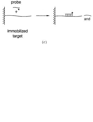
does so, a double-stranded DNA complex will be formed. This

process is called

hy-

bridization,

and all we have to do is to discriminate between this complex and the initial

single-stranded starting materials (Fig. 3.1

a ).

The earliest hybridization experiments were carried out in homogeneous solutions.

Hybridization was allowed to proceed for a fixed time period, and then a physical separa-

tion was performed to capture double-stranded material and discard single strands.

Hydroxyapatite chromatography was used to do this

discrimination because conditions

could be found in which double-stranded DNA bound

to a column

of hydroxylapatite,

while single strands were eluted (Fig. 3.1

b). The amount of double-stranded DNA could

be quantitated by using a radioisotopic label on the

probe or the target, or by measuring

the

bulk amount

of

DNA captured or eluted.

This method is still used today in select

68

ANALYSIS OF DNA SEQUENCES BY HYBRIDIZATION

Ultraviolet absorbance, circular dichroism, or the fluorescence of dyes that bind selec-

tively to duplex DNA can all be used for this purpose. If the amount of double-stranded

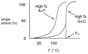
(duplex) DNA in a sample is monitored as a function of temperature, the results typi-

cally obtained are shown in Figure 3.2. The DNA is transformed from double strands at

low temperature, rather abruptly at some critical temperature, to single strands. The

process, for long DNA, is

usually so cooperative that it

can

be likened to

the melting

of

a solid, and the transition is called

DNA

melting.

The midpoint of

the transition for a

particular DNA sample is called the melting temperature,

T m . For DNAs that are very

rich in the bases G

C, this can be 30 or 40°C higher than for extremely (A

T)-rich

samples. It is such spectroscopic observations, on large numbers of

small DNA

du-

plexes that have allowed us to achieve a quantitative

understanding of

most aspects

of

DNA melting.

Figure 3.2

Typical melting

behavior for DNA as a function of average base composition. Shown

is the fraction of single-stranded molecules as a function of temperature. The midpoint of the transi-

tion is the melting temperature,

T

m .

The goal of this section is to define conditions that allow sequence-specific analyses of

DNA using DNA hybridization. Specificity means the ratio of perfectly base-paired du-

plexes to duplexes with imperfections

or

mismatches. Thus

high

specificity means

that

the conditions maximize the amount

of double-stranded perfectly base-paired complex

and minimize the amount of other species. Key

variables are

the concentrations of

the

DNA probes and targets that are used, the temperature, and the salt concentration (ionic

strength).

The melting temperature of long

DNA is concentration

in dependent. This arises from

the way in

which

T m

is

defined. Large DNA melts in patches as shown in

Figure 3.3

a . At

T m , the temperature at which half

the

DNA

is

melted,

(A

T)-rich zones are melted,

while (G

C)-rich zones

are still in duplexes. No net strand separation will have taken

place because no duplexes will have been completely melted. Thus there can be no con-

centration dependence to T

m .

In contrast, the melting of short DNA duplexes, DNAs of 20 base pairs or less, is ef-

fectively all or none (Fig. 3.3

b). In this case the concentration of intermediate species,

partly single-stranded and partly duplex, is sufficiently small that it can be ignored. The

reaction of two short complementary DNA strands,

A

and

B, may be written as

EQUILIBRIA BETWEEN DNA DOUBLE AND SINGLE STRANDS

69

Figure 3.3

Melting behavior of DNA.

(a)Structure of a typical high molecular weight DNA at its

form) is

C

T

. If, for simplicity, all of the strands are initially single stranded, their concen-

trations is

[A ]

[B ]

C

T

o

o

2

At

T m

half

the

strands must be

in

duplex.

Hence

the

concentrations

of

the

different

species at

T

m

will be

[AB ]

[A ] [B ]

C

T

4

The equilibrium constant at

T

m

is

K

a

[AB

]

C

T

/ 4

4

2

[A ][B ] (C T / 4) C T

Do not be misled by this expression into thinking that the equilibrium constant is concen-

tration dependent. It is the

T

m

that is concentration dependent. The equilibrium constant is

temperature dependent. The above expression indicates the value seen for the equilibrium

constant, 4/

C

T , at the temperature,

T m

. This particular

T

m occurs when the equilibrium is

observed at the total strand concentration,

C

T .

70

ANALYSIS OF DNA SEQUENCES BY HYBRIDIZATION

A special case must be considered in which hybridization occurs between two short

single

strands

of the same

identical

sequence,

C.

Such strands are self-complementary.

An example is GGGCCC which can base pair with itself. In this case the reaction can be

written

2C

C

2

The equilibrium constant,

K a , becomes

K a

[C

2]

[C

2

]

At the melting temperature half of the strands must be duplex. Hence

[C 2]

[2C ]

C T

4

where

C T

as before is the total concentration of strands. Thus we can evaluate the equilib-

rium expression at

T m

as

K

a

C T

/ 4

1

(C T / 2)

C

T

As before, what this really means is that

T m

is

concentration dependent.

In both cases

simple mass action considerations ensure that

T m

will increase as the concentration is

raised.

The final case we need to consider is when one strand is in vast excess over the other

instead of both being at equal concentrations. This is frequently the case

when a

trace

amount of probe is used to interrogate a concentrated

sample or, alternatively, when

a

large amount of probe is used to interrogate a very minute sample. The formation of du-

plex can be written as before as

A B

AB

, but now the initial starting conditions are

[B ] [A ]

o

o

Effectively the total strand concentration,

C T

, is thus simply

the initial

concentration of

the excess strand:

B o . At

T m ,

[AB

] [A ]

Thus the equilibrium expression at

T

m

becomes

K

a

[AB

]

1

C T

[A ][B ]

The melting temperature is still concentration dependent.

The importance of our ability to drive duplex formation cannot be

underestimated.

Figure 3.4 illustrates the practical utility of this ability. It shows the concentration depen-

dence

of the melting temperature

of two different duplexes. We can characterize

each re-

THERMODYNAMICS OF THE MELTING OF SHORT DUPLEXES

71

Figure 3.4

The dependence of the

melting temperature,

T m , of two short duplexes on the total

concentration of DNA strands,

C T .

action by its melting temperature and can attempt to extract thermodynamic parameters

like

the

enthalpy

change,

H , and the free energy change,

G

, for

each

reaction.

However, with the

T m ’s

different for the two reactions, if we do this at

T

m , the

thermody-

namic parameters derived will refer to reactions at two different temperatures. There will

be no way, in general, to compare these parameters, since they are expected to be intrinsi-

cally temperature dependent. The concentration dependence of melting saves us from this

dilemma. By varying the concentration, we can produce conditions where the

two du-

plexes

have

the same

T

m . Now thermodynamic parameters derived from each are

compa-

rable. We can, if we wish, choose any temperature for this comparison. In practice, 298 K

has been chosen for this purpose.

THERMODYNAMICS OF THE MELTING OF SHORT DUPLEXES

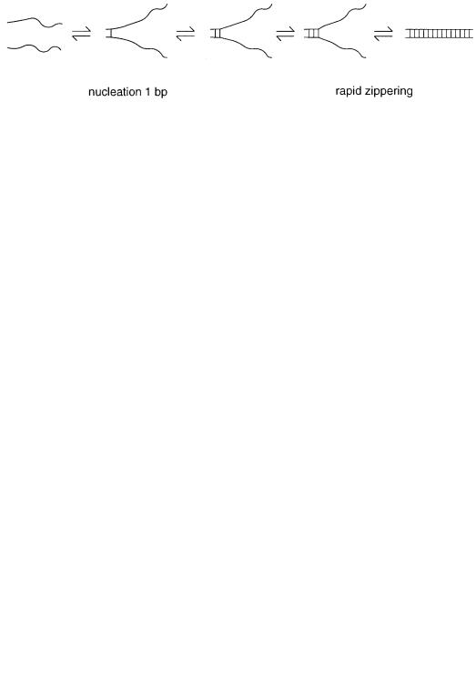
The model we will use to analyze the melting of short DNA double helices is shown in

Figure 3.5. The two strands come

together, in a nucleation step, to form a single pair.

Double strands can form by stacking of adjacent base pairs above or below the initial nu-

cleus until a full duplex has zippered up. It does not matter, in our treatment, where the

initial nucleus forms. We also need

not consider any intermediate steps beyond the nu-

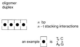
cleus

and the fully

duplex state. In

that state, for a duplex of

n base

pairs,

there will be

n 1 stacking

interactions (Fig.

3.6). Each interaction reflects

the

energetics

of stacking

two adjacent base

pairs on top of

each other. There are ten distinct such

interactions,

as