Добавил:

fench Опубликованный материал нарушает ваши авторские права? Сообщите нам.

Вуз:

Сумский государственный университет

Предмет:

Генетика

Файл:

Genomics- The Science and Technology Behind the Human Genome Project. Charles R. Cantor, Cassandra L / genomics1-10 / 7

.pdf

Скачиваний:

Добавлен:

17.08.2013

Размер:

277.57 Кб

Скачать

☆

1 / 31 2 3 > Следующая >>>

Genomics: The Science and Technology Behind the Human Genome Project.	Charles R. Cantor, Cassandra L. Smith
	Copyright © 1999 John Wiley & Sons, Inc.
	ISBNs: 0-471-59908-5 (Hardback); 0-471-22056-6 (Electronic)

7 Cytogenetics and Pseudogenetics

WHY GENETICS IS INSUFFICIENT

The previous chapter showed the potential power of linkage analysis in locating human disease genes and other inherited traits. However, as demonstrated in the chapter, genetic analysis by current methods is extremely tedious and inefﬁcient. Genetics is the court of

last	resort	when	no	more direct way to locate a	gene of interest is available. Frequently
one	already	has	a	DNA marker believed to be	of interest in the search for a particular

gene, or just of interest as a potential tool for higher-resolution genome mapping. In such cases it is almost always useful to pinpoint the approximate location of this marker within

the genome as rapidly and efﬁciently as possible. This is the realm of cytogenetic and pseudogenetic methods. While some of these have potentially very high resolution, most

often they are used at relatively low resolution to provide the ﬁrst evidence for the chro-

mosomal	and subchromosomal location of a DNA marker of interest. Unlike genetics,
which can work with just a phenotype, most cytogenetics and pseudogenetics are best ac-
complished by direct hybridization using a cloned DNA probe or by PCR.
SOMATIC	CELL GENETICS

In Chapter 2 we described the availability of human-rodent hybrid cells that maintain the full complement of mouse or hamster chromosomes but lose most of their human complement. Such cells provide a resource for assigning the chromosomal location of DNA

probes or PCR products. In the simplest			case a panel of 24 cell lines can be used, each
one containing		only a single human chromosome. In practice, it is more efﬁcient to use
cell	lines that	contain pools of human chromosomes. Then simple binary logic (presence
or absence of a signal) allows the chromosomal location of a probe to be inferred with a
smaller number		of hybridization experiments or PCR ampliﬁcations. In Chapter 9 some
of the principles for constructing pools will be described. However, the general power of
this approach is indicated by the example in Figure 7.1. The major disadvantage of using
pools	is that	they are prone to errors if	the probe in question is not a true single-copy
DNA	sequence	but, in fact, derives from a	gene family with representatives present on

more than one human chromosome. In this case the apparent assignment derived from the

use of pools may be totally erroneous. A second problem with the use of hybrid cells, in general, is the possibility that a given human DNA probe might cross-hybridize with rodent sequences. For this reason it is preferable to measure the hybridization of the probe not by a dot blot but by a Southern blot after a suitable restriction enzyme digestion. The reason for this is that rodents and humans are sufﬁciently diverged that although a similar DNA sequence may be present, there is a good chance that it will lie on a different-sized DNA restriction fragment. This may allow the true human-speciﬁc hybridization to be distinguished from the rodent cross-hybridization.

208

SOMATIC CELL GENETICS

209

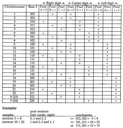
Figure 7.1 Assignment of a cloned DNA probe to a chromosome by hybridization against a panel of cell lines containing limited sets of human chromosomes in a rodent background. This hypotheti-

cal example is based on a base three pooling (see Chapter 9) which is quite efﬁcient compared with randomly selected pools. If the probe is derived from a single chromosome, it can be uniquely assigned. If it contains material that hybridizes to two or more chromosomes, in some cases all of the chromosomes involved can be identiﬁed, but in most cases the results will be ambiguous as shown

by the example at the bottom of the ﬁgure.

An alternative way to circumvent the problem of rodent cross-hybridization in assigning DNA probes to chromosomes is to use ﬂow-sorted human chromosomes, preferably chromosomes that have been sorted from human-rodent hybrid cells so that the puriﬁed

human fraction has very little contamination from other human chromosomes (Chapter

2). This is a very powerful approach; its major limitation is the current scarcity of ﬂowsorted human chromosomal DNA.

210 CYTOGENETICS AND PSEUDOGENETICS

SUBCHROMOSOMAL MAPPING PANELS

Frequently it is possible to assemble sets of cell lines containing fragments of only one chromosome of interest. The occurrences of a DNA probe sequence in a subset of these cell lines can be used to assign the probe to a speciﬁc region of the chromosome. The accuracy of that assignment is determined by the accuracy with which the particular chromosome fragments contained in each cell line are known. This can vary quite considerably, but in general this approach is quite a powerful and popular one. A simple example is shown in Figure 7.2. Here three cell lines are used to divide a chromosome into three regions. The key aspect of these cell lines are breakpoints that determine which chromosome segments are present and which are absent.

A more complex example of cell lines suitable for regional assignment is given in Figure 7.3. Here the properties of a chromosome 21 mapping panel are illustrated. It is evident that some regions of the chromosome are divided by the use of this panel into very high resolu-

tion zones while others are deﬁned much less precisely. In the case shown in Figure 7.3, human cell lines were assembled from available patient material: individuals with translocations or chromosomal deletions. Then these chromosomes were moved by cell fusion into

rodent lines to simplify hybridization analyses. Because no systematic method was used to assemble the panel, the resulting breakpoint distribution is very uneven.

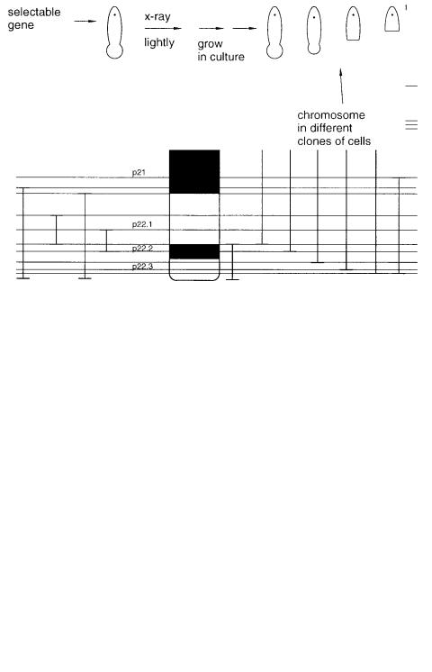
If a selectable marker exists near the end of a chromosome, it is possible to assemble a very orderly and convenient mapping panel. Assuming the selection can be applied in a

hybrid cell, what is done is to irradiate the cell line lightly with X rays so as to cause an average of less than one break per chromosome, and then grow the cells in culture and al-

low broken chromosomes to heal. Since the selection applies to only one end of the human chromosome, there will be a tendency to keep chromosomes containing that end and

lose pieces without that end. The result is a ﬁne, ordered subdivision of the chromosome, as shown in Figure 7.4. This resource is exceptionally useful for mapping the location of cloned probes because the results are usually unambiguous. The pattern of hybridization

should be	a step function and the point where	positive	signal	disappears	indicates the
most distal possible location of the probe.
A few caveats are in order concerning the use of cell lines that derive from broken or
rearranged	human chromosomes. Broken chromosome	are always	healed	by fusion	with

other chromosomes (or by acquisition of telomeres). For example, cell lines described as 21qare missing the long arm of chromosome 21. Frequently such cell lines have other human chromosomes present that have been quietly ignored or forgotten. This is not a problem when a single-copy probe is used, assuming that this probe is already known to

Figure 7.2 A simple example of regional assignment of a DNA sample by hybridization to three cell lines containing incomplete copies of the chromosome of interest. The two break points in the chromosomes are used to divide the chromosome into three intervals.

SUBCHROMOSOMAL MAPPING PANELS

211

Figure 7.3 A mapping panel of hybrid cell lines used to assign probe locations on human chromosome 21. Vertical lines indicate the human chromosome content of each cell line. Note the unevenness of the resulting intervals (horizontal lines).

be located on the chromosome of interest, and the goal is just narrowing down its subchromosomal location. However, the problem is much more serious if the probe of inter-

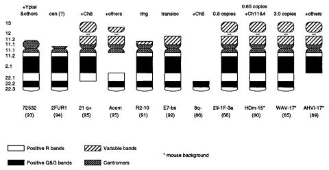
est comes from a gene family or contains repeated sequences. The actual chromosome content of a set of cell lines described as chromosome 21 hybrids is illustrated in Figure 7.5. Many of these lines, in fact, contain other human chromosomes. Cross-hybridization to rodent background is always a potentially serious additional complication when work-

ing with hybrid cells. For this reason it is best to do Southern blots or PCR analysis rather than dot blots, as we already explained earlier in the chapter.

Figure 7.4 A method for selection of broken chromosomes that can be used to generate a much more even mapping panel than the one shown in Figure 7.3.

212 CYTOGENETICS AND PSEUDOGENETICS

Figure 7.5 Actual chromosome content of some of the cell lines used to produce the mapping panel summarized in Figure 7.3. Note that many contain other human chromosomes besides num-

ber 21.

RADIATION

HYBRIDS

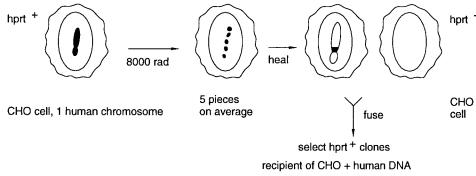
It is possible to make hybrid cells containing small fragments of human chromosomes.

These cell lines represent, essentially, a way of cloning small continuous stretches of hu-

man DNA. The method was originally described by S. Goss and H. Harris, and later re-

discovered and elaborated by D. Cox and R. Meyers (Cox et al., 1990). The basic tech-

nique

for

producing

these

cells,

called

radiation

hybrids,

shown

schematically in

Figure 7.6. The starting point is a hybrid cell line containing only a single human chro-

mosome in a Chinese hamster ovary (CHO) cell with a wild type hypoxanthine ribosyl

transferase (hprt) gene. This cell line is subjected to a very high X-ray dose, 8000 rads,

which is sufﬁcient to break every chromosome into ﬁve pieces on average. After irradia-

tion the fragments are allowed to heal, and the resulting cells are fused with an hprt

CHO

line, one in which an inactive allele of the hprt gene is present. Cell clones that have re-

ceived

and

retained

hprt

DNA are selected and maintained by growth on a particular set

conditions

called

HAT

medium,

which require an active hprt gene. Some

these

clones are recipients of both CHO and human DNA. Note that no human-speciﬁc selec-

tion has been used to focus

the choice of hybrid cells on any particular region of the hu-

man chromosome in question. Thus the population of hybrids should represent a random

sampling of that chromosome if there is no intrinsic selection method operative.

Selection

for

hprt

phenotype ensures that all

the

cell

lines

maintained will

have

been

recipients

some foreign

DNA.

Those

that have human DNA present

can be detected by hybridization with human-speciﬁc

repeated sequences.

Then

these

lines are allowed to grow in the absence

of any selection for human

markers.

This

will

lead to random loss of

human sequences as time progresses. The

cells

are

contin-

ually screened for the presence of human markers until 30% to 60% of the hybrids con-

tain

a particular

marker

interest.

At this

point

the

radiation hybrids contain

quite

few

discrete

fragments of

human

DNA

integrated between

hamster

DNA segments.

RADIATION HYBRIDS

213

Figure 7.6	Steps in the production of a set of	radiation hybrid cell lines. Note that there is no se-
lection for any	of the human DNA fragments, so they	will be lost progressively as the cells are
grown.

They are now used to look at the statistics of co-retention of pairs of human DNA markers. The basic idea is illustrated below, for three markers on a chromosome:

—————A	—— B———————————C——
Even when the chromosome is fragmented into ﬁve pieces, there is a good chance that A
and B will still be found on the same DNA piece; it is much more likely that C will be on
a different piece. Thus cell lines that have lost A are			also likely to have lost				B, but they
are less likely to have lost C. By establishing the presence or absence of particular mark-
ers, we gain information about the relative		proximity	of	the	markers	because	nearby
markers tend to be co-retained.
Here we will examine the statistics of co-retention of marker pairs. There is a basic
problem with this approach. If only two markers at a time are considered, it turns out that
there are more variables than constraints, and approximations have to be used to analyze
the results. With more than two simultaneous markers, the mathematics becomes more
robust but only at a cost of much greater complexity. For didactic purposes we will ana-
lyze the two-marker case; anyone with a serious interest in pursuing this further should be
aware that in practice, one must consider four or more markers at once to avoid the addi-
tional assumptions used later in this section. The parameters we must consider are illus-
trated below. The two markers A and B reside either on the same DNA fragment or on
separate fragments as shown by the horizontal dashed lines. These fragments will have
individual probabilities of retention, as indicated.
————A————B————		retention probability						P	AB
———A———	——B—–—	retention probabilities							P A , P B
The probability that a break has occurred between A and B in a particular irradiation
treatment is given by the additional parameter					. All		four parameters	P A ,	P B , P AB , and
have values between 0 and 1.
What is done experimentally is to examine		a set of hybrid cell clones and					to ask in
each whether markers A and B are	present. The	fraction	of	them	that have	both markers

214 CYTOGENETICS AND PSEUDOGENETICS

present is fAB , the fractions with only A or only B are tion that have retained neither marker is

four parameters by the following equations:

fA and fB , respectively, and the frac- f0 . These four observables can be related to the

	fAB P AB (1 ) P A P B
The	ﬁrst term denotes cells that have maintained A and B on an unbroken piece of DNA;
the	second term considers those cells that have suffered a break between A and B but

have subsequently retained both separate DNA pieces.

fA P A (1 P B )

fB P B (1 P A )

The top equation indicates cells that have had a break between A and B and kept only A; the bottom equation indicates cells with a similar break, but these have retained only B.

f0 (1 P AB ) (1 ) (1 P A ) (1 P B )

The ﬁrst term indicates cells that originally contained

and

a continuous

DNA

piece but subsequently lost this piece (probability 1

P AB ); the second term indicates

cells that originally had a break between A and B and

subsequently lost

both

these

DNA pieces.

The four types of cells represent all possibilities;

fAB fA fB f0 1

This means that we have only three independent observables, but there are four indepen-

dent unknown parameters. The simplest way

around this dilemma would

to assume

that the

probability of retention

individual markers

was

equal,

for

example,

that

P A P

B . However, available experimental data contradict this. Presumably some markers

lie in regions that because of chromosome structural elements like centromeres or telo-

mers, or metabolically active genes, convey a relative advantage or disadvantage for re-

tention of their region. The approximation actually used by Cox and

Myers

allow

analysis of their data is to assume that

and

P B

are related

to the total amount of A and

B retained, respectively:

P A fAB

B fAB

Upon inspection this assumption can be shown to be algebraically false, but in practice, it

seems to work well enough to allow sensible analysis of existing experimental data.

The easiest way to use the two

remaining independent

observables

perform

the

sum indicated below:

fA fB P A (1 P B ) P B (1 P A )

SINGLE-SPERM PCR

215

This can be rearranged to yield a value for

, which is the actual parameter that should be

directly related to the inverse distance between the markers A and B:

fA fB

P A P B 2 P A P B

Here the

parameters

and

B are

evaluated

from

measured

values

fAB , fA , and

fB as

described above.

Note that in using radiation hybrids, one can score any DNA markers A and B whether

they are just physical pieces of DNA or

whether they are inherited traits that can some-

how be detected in the hybrid cell lines.

However,

the

resulting

radiation

hybrid

map,

based on values of

, is expected to be a physical map and not a genetic map. This is be-

cause

is related to the probability of X-ray breakage, which is usually considered to be

a property of the DNA itself and not in any way related to meiotic recombination events.

In most studies to date,

has been assumed to be relatively uniform. This means that in

addition

to marker

order,

estimates

for DNA

distances

between markers were inferred

from measured values of

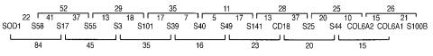
An example of a relatively mature radiation hybrid map, for the long arm of human

chromosome 21, is shown in Figure 7.7. The units of the map are in centirays (cR), where

1 cR is a distance that corresponds to 1% breakage at the X-radiation dosage used. The

density of markers on this

map is impressively high. However, the distances in this map

are not as uniform as previously thought. As shown in Table 7.1, the radiation hybrid map

is considerably elongated at both the telomeric and centromeric edges of the chromosome

arm, relative to the true physical distances revealed by a restriction map of the chromo-

some. It is not known at present whether these discrepancies arose because of the over-

simpliﬁcations used

to construct

the map

(discussed

above)

because,

as has

been

shown in several studies, the probability of breakage or subsequent repair is nonuniform along the DNA. A radiation hybrid map now exists for the entire human genome. It is compared to the genetic map and to physical maps in Table 7.2.

SINGLE-SPERM PCR

A human male will never have a million progeny, but he will have an essentially unlimited number of sperm cells. Each will display the particular meiotic recombination events that generated its haploid set of chromosomes. These cells are easily sampled, but in

Figure 7.7	A radiation hybrid map of part of human chromosome 21. The units of the map are in
centirays (cR). The map shows the order of probes and the		distance	between	each pair. The telo-
mere is to the	right, near S100B. Distances for adjacent	markers	are shown	between the markers,

and for nearest neighbor pairs above and below the map. (Adapted from Burmeister et al., 1994.)

TABLE 7.1	Comparison of the Human Chromosome 21	Not	I Genomic Map
with the Radiation Hybrid Map

Marker Pairs

Physical Distance, kb

cR b

kb/cR a


D21S16–D21S11, 1		5300	2400	87	36	16
D21S11, 1–D21S12		7300	2200	140	52	16
D21S12–SOD		6065	2495	66	92	38
SOD–D21S58		1490	480	22	68	22
D21S58–D21S17		2310	1040	39	59	26
D21S17–D21S55		3860	1600	35	110	46
D21S55–D21S39		3700	1350	43	86	31
D21S39–D21S141, 25		3690	660	40	91	16
D21S151, 25–COL6A		2330	540	54	43	10

Source:	From Wang and Smith (1994).
a The uncertainty shown for each distance is the maximum possible range. The distance given is the mean of that
range. The uncertainty shown for		each ratio is the maximum range, considering only uncertainty in the place-
ment of markers on the restriction map and ignoring any uncertainty in the radiation hybrid map.

b Taken from the data of Cox et al. (1990) and Burmeister et al. (1991). These data were obtained at 8000 rads.

TABLE 7.2	Characteristics of the Human Radiation Hybrid Map
				Average Relative Metrics

Chromosome	Physical Length (Mb)	cM/cR		a	kb/cR a

1	263		0.20		197
2	255		0.21		225
3	214		0.27		233
4	203		0.28		256
5	194		0.29		272
6	183		0.24		243
7	171		0.23		229
8	155		0.26		271
9	145		0.38		305
10	144		0.26		253
11	144		0.30		270
12	143		0.21		234
13q	98		0.22		179
14q	93		0.34		208
15q	89		0.36		203
16	98		0.43		201
17	92		0.23		147
18	85		0.30		172
19	67		0.20		110
20	72		0.30		191
21q	39		0.31		151
22q	43		0.95		185
X	164		0.31		231
Genome	3154		0.31		208

Source: Adapted from McCarthy (1996).

Note: The data were obtained at 3000 rads. Hence physical distances relative to cR are roughly 8/3 as large as the data shown in Table 7.1.

a cM/cR scales the genetic and radiation hybrid maps. kb/cR scales the physical and radiation hybrid maps.

SINGLE-SPERM PCR

217

order to analyze speciﬁc recombination events, it is necessary to be able to examine the

markers

cosegregating in each single sperm cell.

Sperm cannot be biologically ampliﬁed

except by fertilization with an oocyte, and the impracticality of such experiments in the

human is all too apparent. Thus, until in vitro ampliﬁcation became a reality, it was im-

possible to think of analyzing the DNA of single sperm. With PCR, however, this picture

has changed dramatically.

A series of feasibility tests for single-sperm PCR was performed by Norman Arnheim

and co-workers. First they asked whether single diploid human cells could

genotyped

by PCR. They mixed cells from donors who had normal hemoglobin, homozygous for the

gene with cells from donors who had sickle cell anemia, homozygous for the

gene.

Single cells were selected by micromanipulation and were tested by PCR ampliﬁcation of

the

locus followed by hybridization of a dot blot with allele-speciﬁc oligonucleotide

probes. The purpose of the experiment was to determine whether the pure alleles could be

detected

reliably, or whether there would

be cross-contamination between

the

two types

of cells. The results for 37 cells analyzed were 19

A , 12

S , 6 none, and 0 both. This was

very encouraging.

The next test involved the analysis of single

sperm

from

donors

with two

different

LDL receptor alleles. For 80 sperm analyzed, the results were 22 allele 1, 21 allele 2, 1

both alleles, and the remainder neither allele. Thus the efﬁciency of the single-sperm

analysis

was less than with diploid cells, but

the cross-contamination

level

was low

enough to be easily dealt with. A ﬁnal test was to look at two nonlinked two-allele sys-

tems. One was on chromosome 6 (a

or a

2 ), and

the

other

chromosome 19

or b 2 ).

Four types of gametes were expected in equal ratios. What was actually observed is

a 1b 1

a 1b 2

a 2 b 1

a 2 b 2

This is really quite close to what was expected statistically,

The ﬁnal step was to do single-sperm linkage studies. In this case one does simultane-

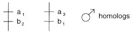
ous PCR analyses on linked markers. Consider the example shown in Figure 7.8. Nothing

needs to be known about the parental haplotypes to start with. PCR

analysis

automati-

cally provides the parental phase. In the case shown in the ﬁgure, most of the sperm mea-

sured at loci a and b have either alleles a

1 and b

or a

3 and b

1. This indicates that these are

the haplotypes of the two homologous chromosomes in the donor. Occasional recombi-

nants

are

seen with alleles a

1 and b

1 or a

3 and

2 . The frequency

at which

these

are ob-

served is a true measure of the male meiotic recombination frequency between markers a and b. Since large numbers of sperm can be measured, one can determine this frequency very accurately. Perhaps more important, with large numbers of sperm, very rare meiotic

recombination events can be detected, and thus very short genetic distances can be measured.

Figure 7.8 Two unrecombined homologous chromosomes that should predominate in the sperm expected from a hypothetical donor. Note that the observed pattern of alleles also determines the phase at these loci if it is not known in advance.

1 / 31 2 3 > Следующая >>>

Соседние файлы в папке genomics1-10

#
17.08.2013435.19 Кб502.pdf
#
17.08.2013343.56 Кб463.pdf
#
17.08.2013296.13 Кб464.pdf
#
17.08.2013326.85 Кб455.pdf
#
17.08.2013406.31 Кб456.pdf
#
17.08.2013277.57 Кб467.pdf
#
17.08.2013634.83 Кб478.pdf
#
17.08.2013475.69 Кб469.pdf
#
17.08.2013192.47 Кб48booktext[1].pdf