Добавил:

fench Опубликованный материал нарушает ваши авторские права? Сообщите нам.

Вуз:

Сумский государственный университет

Предмет:

Генетика

Файл:

Genomics- The Science and Technology Behind the Human Genome Project. Charles R. Cantor, Cassandra L / genomics1-10 / 8

.pdf

Скачиваний:

Добавлен:

17.08.2013

Размер:

634.83 Кб

Скачать

☆

1 / 61 2 3 4 5 6 > Следующая >>>

Genomics: The Science and Technology Behind the Human Genome Project.	Charles R. Cantor, Cassandra L. Smith
	Copyright © 1999 John Wiley & Sons, Inc.
	ISBNs: 0-471-59908-5 (Hardback); 0-471-22056-6 (Electronic)

8 Physical Mapping

WHY HIGH-RESOLUTION PHYSICAL MAPS ARE NEEDED
Physical maps are needed because ordinary human genetic maps are	not detailed enough
to allow the DNA that corresponds to particular genes to be isolated efﬁciently. Physical
maps are also needed as the source for the DNA samples that can serve as the actual sub-
strate for large-scale DNA sequencing projects. Genetic linkage	mapping provides a set
of ordered markers. In experimental organisms this set can	be almost as dense as one
wishes. In humans one is much more limited because of the inability to control breeding
and produce large numbers of offspring. Distances that emerge from human genetic map-
ping efforts are vague because of the uneven distribution of meiotic recombination events

across the genome. Cytogenetic mapping, until recently, was low resolution; it is improving now, and if it were simpler to automate, it could well provide a method that would supplant most others. Unfortunately, current conventional approaches to cytogenetic map-

ping seem difﬁcult to automate, and they are slower than many other approaches that do not involve image analysis.

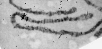
It is worth noting here that in some other organisms, cytogenetics is more powerful than in the human. For example, in Drosophila the presence of polytene salivary gland chromosomes provides a tool of remarkable power and simplicity. The greater extension

and higher-resolution imaging of polytene chromosomes allows bands to be seen at a typ-

ical resolution of 50 kb (Fig. 8.1). This is more than 20 times the resolution in the best human metaphase FISH. Furthermore the large number of DNA copies in the metaphase

salivary chromosomes means that microdissection and cloning are much more powerful

here than they are in the human. It would be nice if there were a convenient way to place large continuous segments of human DNA into Drosophila and then use the power of the cytogenetics in this simple organism to map the human DNA inserts.

Radiation hybrids offer, in principle, a way to measure distances between markers accurately. However, in practice, the relative distances in radiation hybrid maps appear to be distorted (Chapter 7). In addition there are a considerable number of unknown features of


these cells; for example, the			types	of unseen	DNA rearrangements that may be present
need to be characterized. Thus it			is not	yet clear	that the use of radiation hybrids	alone
can	produce a complete	accurate map or yield a set			of DNA samples worth subcloning
and	characterizing at	higher resolution. Instead,			currently other methods must be used	to

accomplish the three major goals in physical mapping:

1.Provide an ordered set of all of the DNA of a chromosome (or genome).

2.Provide accurate distances between a dense set of DNA markers.

3.Provide a set of DNA samples from which direct DNA sequencing of the chromo-

some or genome is possible. This is sometimes called a

sequence-ready map.

234

RESTRICTION MAPS

235

Figure 8.1 Banding seen in polytene Drosophila salivary gland chromosomes. Shown is part of chromosome 3 of for which a radiolabeled probe to the gene for heat-shock protein hsp70 has been hybridized. A strong and weak site are seen. (Figure kindly provided by Mary Lou Pardue.)

Most workers in the ﬁeld focus their efforts on particular chromosomes or chromosome regions. Usually a variety of different methods are brought to bear on the problems

of isolating clones and probes and using these to order each other and ultimately produce ﬁnished maps. However, some research efforts have produced complete genomic maps with a restricted number of approaches. Such samples are turned over to communities interested in particular regions or chromosomes that ﬁnish a high-resolution map of the regions of interest.

There are basically two kinds of physical maps commonly used in genome studies: restriction maps and ordered clone banks or ordered libraries. We will discuss the basic methodologies used in both approaches separately, and then, in Chapter 9, we will show how the two methods can be merged in more powerful second generation strategies. First

we outline the relative advantages and disadvantages of each type of map.

RESTRICTION MAPS

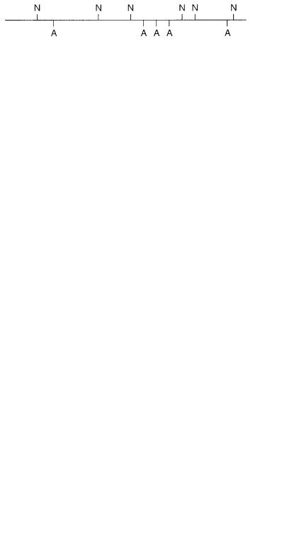
A typical restriction map is shown in Figure 8.2. It consists of an ordered set of DNA fragments that can be generated from a chromosome by cleavage with restriction enzymes individually or in pairs. Distances along the map are known as precisely as the lengths of the DNA fragments generated by the enzymes can be measured. In practice,

the	lengths are measured	by electrophoresis in virtually all currently used methods;
they	are accurate to a	single base pair up to DNAs around around 1 kb in sizes.

Lengths can be measured with better than 1% accuracy for fragments up to 10 kb, and

with a low percent of accuracy for fragments up to 1 Mb		in size. Above this length,
measurements today are still fairly qualitative,	and it is	always best to try to subdivide
a target into pieces less than 1 Mb before any	quantitative claims are made about its
true total size.

236 PHYSICAL MAPPING

Figure 8.2 Typical section of a restriction map generated by digestion of genomic or cloned DNA with two enzymes with different recognition sites A, and N.

In an ideal restriction map each DNA fragment is pinned			to markers on other maps.
Note that	if this is	done with randomly chosen probes,	the locations of these probes
within each	DNA fragment	are generally unknown (Fig. 8.3).	Probes that correspond to

the ends of the DNA fragments are more useful, when they are available, because their position on the restriction map is known precisely. Originally probes consisted of unsequenced DNA segments. However, the power of PCR has increasingly favored the use of sequenced DNA segments.

A major advantage of a restriction map is that accurate lengths are known between sets of reference points, even at very early stages in the construction of the map. A second advantage is that most restriction mapping can be carried out using a top-down strategy that

preserves an overview of the target and that reaches a nearly	complete	map relatively
quickly. A third advantage of restriction mapping is that one	is working	with genomic
DNA fragments rather than cloned DNA. Thus all of the potential artifacts that can arise
from cloning procedures are avoided. Filling in the last few small pieces is always a chore

in restriction mapping, but the overall map is a useful tool long before this is accomplished, and experience has shown that restriction maps can be accurately and completely constructed in reasonably short time periods.

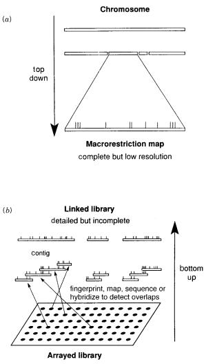
In top-down mapping one successively divides a chromosome target into ﬁner regions and orders these (Fig. 8.4). Usually a chromosome is selected by choosing a hybrid cell in which it is the only material of interest. There have been some concerns about the use of

hybrid cells as the source of DNA for mapping projects. In a typical hybrid cell there is no compelling reason for the structure of most of the human DNA to remain intact. The biological selection that is used to retain the human chromosome is actually applicable to

only a single gene on it. However, the available results, at least for chromosome 21, indicate that there are no signiﬁcant differences in the order of DNA markers in a selected set

of hybrid and human cell lines (see Fig. 8.49). In a way this is not surprising; even in a human cell line most of the human genome is silent, and if loss or rearrangement of DNA

were facile under these circumstances,	it should have been observed. Of course, for
model organisms with small genomes, there is no need to resort to a hybrid cell at all—
their genomes can be studied intact, or the chromosomes can be puriﬁed in bulk by PFG.
In a typical restriction mapping effort, any preexisting genetic map information can be
used as a framework for constructing the physical map. Alternatively, the chromosome of
interest can be divided into regions by	cytogenetic methods or low-resolution FISH.

Figure 8.3 Ambiguity in the location of a hybridization probe on a DNA fragment.

RESTRICTION MAPS

237

Figure 8.4	Schematic	illustration of methods used in physical mapping. (	a ) Top-down strategy
used in restriction mapping. (		b ) Bottom-up strategy used in making an ordered library.

Large DNA fragments are produced by cutting the chromosome with restriction enzymes

with very rare recognition sites. The fragments are separated by size and assigned to re-

gions by hybridization with genetically or cytogenetically mapped DNA probes. Then the

fragments are assembled into contiguous blocks, by

methods that will be described

later

in this chapter. The result at this point

called

macrorestriction map.

The fragments

may average 1 Mb in size. For a simple genome this means that only 25 fragments will

have to be ordered. This is relatively straightforward. For an intact human genome, the

corresponding number is 3600 fragments. This is an

unthinkable

task unless

the frag-

ments are ﬁrst assorted into individual chromosomes.

If a ﬁner

map

is desired, it

can

be constructed by taking

the

ordered

fragments

one

at a time,

and

dissecting these

with

frequently

cutting

restriction

nucleases.

238			PHYSICAL		MAPPING
advantage		of	this reductionist mapping approach is that the ﬁner maps can be made only
in	those regions where there is sufﬁcient interest to justify this much more arduous task.
	The major disadvantage of most restriction mapping efforts is that they do not produce
the	DNA	in	a	convenient, immortal		form	where	it can be distributed or sequenced
by	available methods. One could try to clone the large DNA fragments that compose
the	macrorestriction map, and there has been some progress in developing the vectors
and	techniques			needed	to do this. One could also use PCR				to	generate segments of
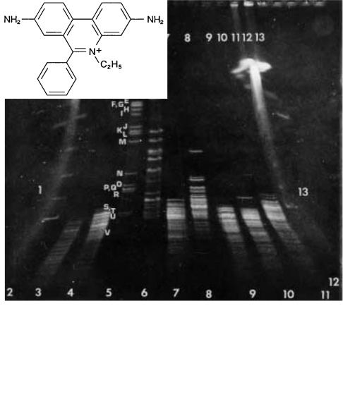
these large fragments (see Chapter 14). For a small genome, most of the macrorestriction
fragments it contains can usually be separated and puriﬁed by a single PFG fractionation.
An	example		is	shown	in Figure 8.5.	In	cases	like this,	one	does really possess the

Figure 8.5 Example of the fractionation of a
restriction		enzyme	digest	of	an	entire	small
genome	by	PFG.		Above:		Not		I digest of	the
4.6	Mb	E. coli	genome		shown	in lane		5;	Sﬁ I
digest	in	lane 6.	Other		lanes	shown	enzymes
that cut too frequently to				be useful for				map-
ping. (Adapted from Smith et al., 1987.)									Left:
Structure of the ethidium cation used to stain the
DNA fragments.

ORDERED LIBRARIES

239

genome, but it is not in a form where it is easy to handle by most existing techniques. For a large genome, PFG does not have sufﬁcient resolution to resolve individual macrore-


striction fragments. If one starts instead with a hybrid					cell, containing only a single hu-
man chromosome or chromosome fragment, most of the				human macrorestriction frag-
ments will be separable from one another. But they will					still be contaminated, each by
many other background fragments from the rodent host.
ORDERED		LIBRARIES
Most genomic libraries are made by partial digestion with a relatively frequently cutting
restriction		enzymes, size selection of the fragments			to provide a fairly uniform set of
DNA inserts, and then cloning these into a vector appropriate for the size range of inter-
est. Because of the method by which			they were produced, the cloned fragments are a
nearly random set of DNA pieces. Within the library, a given small DNA region will be
present on many different clones. These extend to varying degrees on both sides of the
particular region (Fig. 8.6). Because the clones					contain overlapping regions of the
genome, it is possible to detect these overlaps by various ﬁngerprinting methods that ex-
amine patterns of sequence on particular clones. The random nature of the cloned frag-
ments means that many more clones exist than the minimum set necessary to cover the
genome. In practice, the redundancy of the library is usually set at ﬁveto tenfold in order
to ensure that almost all regions of the genome will have been sampled at least once (as
discussed in Chapter 2). From this vast library the goal is to assemble and to order the
minimum set of clones that covers the genome in one contiguous block. This set is called
the	tiling path.
	Clone libraries have usually been ordered by a bottom-up approach. Here individual
clones are initially selected from the			library at random. Usually the library is handled as
an array of samples so that each clone has a unique location on a set of microtitre plates,
and the chances of accidentally confusing two different					clones can be minimized. The
clone is ﬁngerprinted, by hybridization, by restriction mapping, or by determining bits of
DNA sequence. Eventually clones appear that share some or all of the same ﬁngerprint
pattern (Fig. 8.7). These are clearly overlapping, if not identical, and they are assembled
into	overlapping sets, called		contigs,	which is short for contiguous blocks. There are sev-
eral obvious advantages to this approach. Since the DNA is handled as clones, the map is
built up of immortal samples that are			easily distributed		and that are potentially suitable
for direct sequencing. The maps are usually fairly high resolution when small clones are
used, and some forms of ﬁngerprinting provide very				useful internal information about
each clone.


Figure 8.6		Example of a dense library of clones. (		a ) The large number of clones insures that a
given DNA probe or region (vertical			dashed line) will occur on quite a few different clones in the li-
brary. (	b ) The minimum tiling		set is the smallest number of clones that can be selected to span the
entire sample of DNA.

240 PHYSICAL MAPPING

Figure 8.7	Example of a bottom-up	ﬁngerprinting strategy	to order	a dense set of clones. (	a ) A
clone is selected at random and ﬁngerprinted. (			b )	Two clones that share an overlapping ﬁngerprint
pattern are assembled into a contig. (		c ) Longer	contigs	are assembled as more overlapping	clones
are found.

There

are a

number

of disadvantages to bottom-up

mapping.

While

this

process

easy to automate, no overview of the

chromosome

or genome is

provided

the

ﬁngerprinting

and

contig

building. Additional experiments have to

done

place

contigs on

lower-resolution framework map, and most approaches do

not necessarily

allow the

orientation of

each contig to be

determined

easily. A

serious

limitation

of pure bottom-up mapping strategies is that they do not reach completion. Even if the original library is a perfectly even representation of the genome, there is a statistical prob-

lem	associated with the random clone picking used. After a while, most new clones	that
are	picked will fall into contigs that are already saturated. No new information	will be

gained from the characterization of these new clones. As the map proceeds, a diminishingly smaller fraction of new clones will add any additional useful information. This problem becomes much more serious if the original library is an uneven sample of the chromosome or genome. The problem can be alleviated somewhat if mapped contigs are

used to screen new clones prior to selection to try to discard those that cannot yield new information. An additional ﬁnal problem with bottom-up maps is shown in Figure 8.8.

Usually the overlap distance between two	adjacent members of	a	contig	is not known
with much precision. Therefore distances	on a typical bottom-up		map are	not	well de-
ﬁned.
The number of samples or clones that must be handled in top-down or bottom-up mapping
projects can be daunting. This number also	scales linearly with	the	resolution		desired. To

gain some perspective on the problem, consider the task of mapping a 150-Mb chromosome.

Figure 8.8 Ambiguity in the degree of clone overlap resulting from most ﬁngerprinting or clone ordering methods.

RESTRICTION NUCLEASE GENOMIC DIGESTS

241

This is the average size of	a human chromosome. The	numbers of samples needed are
shown below:
RESOLUTION	RESTRICTION MAP		ORDERED LIBRARY	(5 REDUNDANCY	)
1 Mb	150 fragments		750 clones
0.1 Mb	1500 fragments		7500 clones
0.01 Mb	15,000 fragments		75,000 clones
With existing methods the current convenient range for constructing physical maps of en-
tire human chromosomes allows a resolution of somewhere between 50 kb (for the most
arduous bottom-up approaches attempted) to 1 Mb for much easier restriction mapping or
large insert clone contig building.
The resolution desired in a map will determine the sorts of clones that are conveniently
used in bottom-up approaches. Among the possibilities currently available are
Bacteriophage lambda			10 kb inserts
Cosmids			40 kb inserts
P1 clones			80 to 100 kb inserts
Bacterial artiﬁcial chromosomes (BACs)			100 to 400 kb inserts
Yeast artiﬁcial chromosomes (YACs)			100 to 1300 kb inserts
The ﬁrst three types of clones can be easily grown in			large numbers of copies per cell.
This greatly simpliﬁes DNA preparation, hybridization, and other analytical procedures.
The last two types of clones are usually handled as single copies per host cell, although
some methods exist for amplifying them. Thus they are more difﬁcult to work with, indi-
vidually, but their larger insert size makes low-resolution mapping much more rapid and
efﬁcient.
RESTRICTION NUCLEASE GENOMIC	DIGESTS
Generating DNA fragments of the desired size range is critical for producing useful li-
braries and genomic restriction maps. If genomes were statistically random collections of
the four bases, simple binomial statistics would allow us to estimate the average fragment
length that would result from a given restriction nuclease recognition site in a total digest.
For a genome where each of the four bases is equally represented, the probability of oc-
currence of a particular site of size		n	is 4 n ; therefore the average fragment length gener-
ated by that enzyme will be 4	n . In practice, this becomes
	SITE SIZE (N )		AVERAGE FRAGMENT LENGTH	(kb)
	4		1
	6		4
	8		64
	10		1000

242

PHYSICAL

MAPPING

This tabulation indicates that enzymes with four or six base sites are convenient for the

construction of partial digest small insert libraries. Enzymes with sites

ten bases

long

would be the preferred choice for low-resolution macrorestriction mapping, but such en-

zymes are unknown. Enzymes with eight-base sites would be most useful for currently

achievable large-insert cloning. More accurate schemes for predicting cutting frequencies

are discussed in Box 8.1.

A list of the enzymes currently available that have relatively rare cutting sites in mam-

malian genomes is given in Table 8.1. Unfortunately, there are only a few known restriction

enzymes with eight-base speciﬁcity, and most of these have sites that are not well-predicted

by random statistics. A few enzymes are known with larger recognition sequences. In most

cases there is not yet convincing evidence that the available

preparations of

these

enzymes

have low enough contamination with random nonspeciﬁc nucleases to allow them to be used

for a complete digest to generate a discrete nonoverlapping

set of large DNA fragments.

Several enzymes exist that have sites so rare that they

will not occur at all

natural

genomes. To use these enzymes, one must employ strategies in which the sites are introduced

into the genome, their location is determined, and then cutting at the site is used to generate

fragments containing segments of the region where the site was inserted. Such strategies are

potentially quite powerful, but they are still in their infancy.

The unfortunate conclusion, from experimental studies on the pattern of DNA fragment

lengths generated by genomic restriction nuclease digestion,

is that most currently available

8-base speciﬁc enzymes are not useful for generating fragments suitable for macrorestriction

mapping. Either the average fragment length is too short, or the digestion is not complete,

leading to an overly complicated set of reaction products. However, mammalian genomes are

very poorly modeled by binomial statistics,

and

thus

some

enzymes,

which

statistically

might be thought to be useless because they would generate fragments that are too small, in

fact generate fragments in useful size ranges. As a speciﬁc example, consider the ﬁrst two en-

zymes known with eight-base recognition sequences:

Sﬁ

GGCCN^NNNNGGCC

Not

GC^GGCCGC

Here the symbol N indicates that any of the four bases can occupy this site; the caret (^)

indicates the cleavage site on the strand shown; there is

corresponding site

on the sec-

ond strand.

Human

DNA

is A–T

rich; like that of other

mammals

contains approximately

60%

A T. When this is factored into the predictions (Box 8.1), on the basis of base composi-

tion, alone, these enzymes would be expected to cut human DNA every 100 to 300 kb. In

fact

Sﬁ

I digestion of the human genome yields DNA fragments that predominantly range

in size from 100 to 300 kb. In contrast,

Not

I generates

DNA

fragments that average

closer to 1 Mb in size. The size range generated by

Sﬁ

I would make it potentially useful

for some applications, but the cleavage speciﬁcity of

Sﬁ

I leads to some unfortunate com-

plications. This enzyme cuts within an unspeciﬁed sequence. Thus the fragments it gener-

ates cannot be directly cloned in a straightforward manner

because the three base over-

hang

generated

Sﬁ I is

a mixture

of 64 different sequences. Another problem,

introduced by the location of the

Sﬁ

I cutting site, is

that different

sequences

turn out

be cut at very different rates. This makes it difﬁcult to achieve total digests efﬁciently, and

as described later, it also makes it very difﬁcult to use

Sﬁ

I in

mapping

strategies

that de-

pend on the analysis of partial digests.

RESTRICTION NUCLEASE GENOMIC DIGESTS

243

BOX 8.1

PREDICTION OF RESTRICTION ENZYME-CUTTING FREQUENCIES

An accurate prediction of cutting			frequencies requires an accurate statistical estima-
tion of the probability of occurrence of the enzyme recognition site. To accomplish
this, one must take into account two factors: First, the sample of interest, that is, the
human genome, is unlikely to have a base composition that is precisely 50% G					C,
50% A T. Second,		the	frequencies of particular dinucleotide sequences often vary
quite substantially from that predicted by simple binomial statistics based on the base
composition. A rigorous treatment should also take the mosaicism into account (see
Chapters 2 and 15).
Base composition effects alone can be considered, for double-stranded DNA with a
single variable:	X G	C	1 X A T , where X is a mole fraction. Then the expected fre-
quency of occurrence of a site with			n G’s or C’s and	m	A’s or T’s is just

	2
	1	n m (X G	C )n (1 X G C )m
		n m (X G	C )n (1 X G C )m
To take base sequence into account, Markov statistics can be used. In Markov chain
statistics the probability of the		n th event in a		series can	be	inﬂuenced by the		speciﬁc
outcome of the prior events such as the	(		n	1)th	and	(	n 2)th	events. Thus Markov
chain statistics can take into account known frequency information about the occur-
rences of sequences of events. In other	words, this kind		of statistics		is ideally		suited
for the analysis of sequences.
Suppose that the frequencies of particular dinucleotide sequences are known for the
sample of interest. There are 16 possible dinucleotide sequences: The frequency								X A,C,
for example, indicates the fraction	of dinucleotides that has a AC sequence on						one
strand base paired to a complementary GT on the other. The sum of these frequencies
is 1. Only 10 of the 16 dinucleotide sequences are distinct unless we consider the two
strands separately. On each strand, we can relate dinucleotide and mononucleotide fre-
quencies by four equations:
	X A,C X A,A		X A,T X A,G X A

since base A must always be followed by some other base (the X’s indicate mole fraction). The expected frequency of occurrence of a particular sequence string, based on these nearest-neighbor frequencies is just

	n	X i,i 1
	X 12
		X i
	i 2
where the product is taken successively over the mole fractions
X i of all successive dinucleotides	i,i 1, and mononucleotides

terest. Predictions done in this way are usually more accurate than predictions based

solely on the base composition. Where		methylation occurs that can block the cutting
of	certain restriction nucleases, the	issue becomes much more complex, as discussed
in	the text.

X i,i 1 , respectively, and i in the sequence of in-

1 / 61 2 3 4 5 6 > Следующая >>>

Соседние файлы в папке genomics1-10

#
17.08.2013343.56 Кб463.pdf
#
17.08.2013296.13 Кб464.pdf
#
17.08.2013326.85 Кб455.pdf
#
17.08.2013406.31 Кб456.pdf
#
17.08.2013277.57 Кб467.pdf
#
17.08.2013634.83 Кб478.pdf
#
17.08.2013475.69 Кб469.pdf
#
17.08.2013192.47 Кб48booktext[1].pdf