

74 ANALYSIS OF DNA SEQUENCES BY HYBRIDIZATION
BOX 3.3
STACKING PARAMETERS AT OTHER TEMPERATURES
In practice, it turns out to be a sufficiently accurate approximation to assume that the
various |
H s0are'sindependent of temperature. This is a considerable simplification. It |
allows direct integration of the van’t Hoff relationship to compute thermodynamic parameters at any desired temperature from the parameters measured at 298 K. Starting from the usual relationship for the dependence of the equilibrium constant on temperature,
|
d (ln K ) |
|
|
d (1 /T ) |
|
we can integrate this directly: |
|
|
|
|
R |
|
d (ln K ) |
H |
H 0
R
0 d T1
With |
limits of integration |
from |
T 0 , which is 298 K, to |
|
any other |
melting temperature, |
||||||
T m |
, the result is |
|
|
|
|
|
|
|
|
|
|
|
|
|
|
ln K (T m |
) ln K (T 0 ) |
H 0 |
1 |
|
1 |
|
|||
|
|
|
|
|
|
|
|
|
||||
|
|
|
R |
|
T m |
T 0 |
||||||
|
|
|
|
|
|
|
|
|||||
However, the first term of the left-hand side of the equation, for a pair of complemen- |
|
|
|
|
||||||||
tary |
oligonucleotides, |
is |
just 4/ |
C T . The second term on the |
left-hand side is equal to |
|||||||
G |
(T 0 )/RT 0 . Inserting these values and rearranging gives a final, useful expression for |
|||||||||||
computing the |
T m |
of a duplex at any temperature from data measured at 298 K. All of |
||||||||||
the necessary data are summarized in Table 3.1. |
|
|
|
|
|
|
|
|
|
|||
T m
T 0
H
0
G
H 0
0 (T 0 ) RT 0 ln( C T / 4)
THERMODYNAMICS OF IMPERFECTLY PAIRED DUPLEXES |
|
|
|
|
|||
In contrast to the small number of discrete interactions that must be considered in calcu- |
|
||||||
lating the energetics of perfectly paired DNA duplexes, there is a plethora of ways that |
|
|
|||||
duplexes can pair imperfectly. We have available model compound data on most |
of |
these |
|
|
|||
so that estimates of the energetics can be made. However, the large number of possibili- |
|
|
|||||
ties precludes a complete analysis of imperfections in the context of |
all |
possible |
se- |
|
|||
quences, at least for the present. |
|
|
|
|
|
|
|
The simplest imperfection is a dangling end, as shown in Figure 3.7 |
|
|
a. |
If both ends are |
|||
dangling, their contributions can be treated separately. From available data |
it |
appears that |
|
||||
a dangling |
end contributes |
8 kcal/mol on average to |
the overall |
H of |
duplex forma- |
||
tion, and |
1 kcal/mol to the |
overall |
G of duplex |
formation. The |
large enthalpy arises |
|
|
|
THERMODYNAMICS OF IMPERFECTLY PAIRED DUPLEXES |
75 |
|||||
TABLE |
3.2 Predicted and Observed Stabilities |
|
|
|
|
||
(free energy of formation) of Various |
|
|
|
|
|
|
|
Oligonucleotide Duplexes |
|
|
|
|
|
|
|
|
|
|
|
|
|
|
|
Comparison of Calculated and Observed |
|
|
G |
(kcal/mol) |
|
||
|
|
|
|
|
|
|
|
|
Oligomeric Duplex |
|
G |
pred |
G obs |
|
|
|
|
|
|
|
|
|
|
1 |
GCGCGC |
|
11.1 |
|
11.1 |
|
|
|
CGCGCG |
|
|
|
|
|
|
2 |
CGTCGACG |
|
11.2 |
11.9 |
|
|
|
|
GCAGCTGC |
|
|
|
|
|
|
3 |
GAAGCTTC |
|
7.9 |
|
8.7 |
|
|
|
CTTCGAAG |
|
|
|
|
|
|
4 |
GGAATTCC |
|
9.3 |
|
9.4 |
|
|
|
CCTTAAGG |
|
|
|
|
|
|
5 |
GGTATACC |
|
6.7 |
|
7.4 |
|
|
|
CCATATGG |
|
|
|
|
|
|
6 |
GCGAATTCGC |
|
16.5 |
15.5 |
|
|
|
|
CGCTTAAGCG |
|
|
|
|
|
|
7 |
CAAAAAG |
|
6.1 |
|
6.1 |
|
|
|
GTTTTTC |
|
|
|
|
|
|
8 |
CAAACAAAG |
|
9.3 |
10.1 |
|
|
|
|
GTTTGTTTC |
|
|
|
|
|
|
9 |
CAAAAAAAG |
|
9.9 |
9.6 |
|
|
|
|
GTTTTTTTC |
|
|
|
|
|
|
10 |
CAAATAAAG |
|
8.5 |
8.5 |
|
|
|
|
GTTTATTTC |
|
|
|
|
|
|
11 |
CAAAGAAAC |
|
9.3 |
9.5 |
|
|
|
|
GTTTCTTTC |
|
|
|
|
|
|
12 |
CGCGTACGCGTACGCG |
32.9 |
34.1 |
|
|
|
|
|
GCGCATGCGCATGCGC |
|
|
|
|
|
|
|
|
|
|
|
|||
Note: Calculations use the equations given in the text and the mea- |
|
|
|
|
|||
sured thermodynamic values given in Table 3.1. |
|
|
|
|
|
|
|
Source: |
Adapted from Breslauer et al. (1986). |
|
|
|
|
||
because the first base of the dangling end can still stack on the |
last base pair of the |
du- |
|
|
|||||||
plex. Note that there are two distinct types of dangling ends: a 3 |
|
|
|
|
|
-overhang and a 5 |
-over- |
||||
hang. At the current level of available information, we treat these as equivalent. Simple |
|
|
|||||||||
dangling ends will arise whenever a target and a probe are different in size. |
|
|
|
|
|
||||||
The next imperfection, which leads to considerable destabilization, is an internal mis- |
|
|
|||||||||
match. As |
shown |
in Figure |
3.7 |
b, this leads to the |
loss |
of two internal |
and two inH- s0 's |
|
|||
ternal |
G |
s0 'sApparently. this is empirically compensated by some |
residual |
stacking |
ei- |
|
|
||||
ther between the bases that are mispaired and the duplex borders or between the bases |
|
|
|
||||||||
themselves. Whatever the detailed mechanism, the result is to |
gain |
back |
about |
|
|
8 |
|||||
kcal/mol |
in |
H. |
There is no effect on the |
G. |
A larger internal mismatch is called an |
|
|||||
internal |
loop. |
Considerable data on the thermodynamics of |
such loops exist for RNA, |
|
|
||||||
and much |
less |
for DNA. In general, such structures will be |
far less stable than the |
|
|
||||||
perfect duplex |
because of |
the loss |
of additional free energies and |
enthalpies of |
stacking. |
|
|
||||
76 ANALYSIS OF DNA SEQUENCES BY HYBRIDIZATION
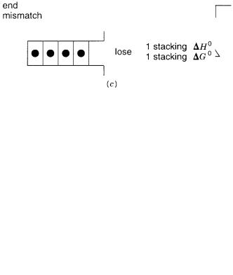
Figure 3.7 |
Stacking interactions |
in various types of imperfectly matched duplexes. |
(a)Dangling |
|
ends. |
(b)Internal mismatch. |
(c)Terminal mismatch. |
|
|
A related imperfection is a bulge loop in which two strands of unequal size come together |
|
|
|
||||||||
so that one is perfectly paired while the other has an internal loop of unpaired residues. |
|
|
|
||||||||
There |
can |
also |
be internal loops in which the single-stranded |
regions are of different |
|
|
|
||||
length on the two strands. Again the data describing the thermodynamics of such struc- |
|
|
|
||||||||
tures are available mostly just for RNAs (Cantor and Schimmel, 1981). There are many |
|
|
|
||||||||
complications. See, for example, Schroeder et al. (1996). |
|
|
|
|
|||||||
A key imperfection that needs to be |
considered |
to understand the specificity of |
|
|
|
||||||
hybridization is |
a terminal |
mismatch. As shown |
in Figure |
3.7 |
c, this |
results in |
the |
loss of |
|||
one |
H |
0 |
one |
0 |
an external mismatch |
should be |
less destabilizing than an |
|
|
|
|
and |
. SuchG |
|
|
|
|||||||
|
|
s |
|
s |
|
|
|
|
|
|
|
internal mismatch because one less stacking interaction is disrupted. It is not clear, at the |
|
|
|
||||||||
present time, how much any stacking of the mismatch to the end of the duplex partially |
|
|
|
||||||||
compensates for the lost duplex stacking. It may be adequate to model an end-mismatch |
|
|
|
||||||||
like |
a dangling |
end. Alternatively, one might consider it like an internal mismatch with |
|
|
|
||||||
only one lost set of duplex stacking interactions. Both of these cases require no correction |
|
|
|
||||||||
to the predicted |
G of duplex formation, once the lost stacking interactions have been ac- |
|
|
|
|||||||
counted for. Therefore at present it is simplest to concentrate on |
G |
estimates |
and |
ignore |
|||||||
H |
estimates. More studies are needed in this area to clear up these uncertainties. In |
|
|
|
|||||||
Chapter 12 we will discuss attempts to use hybridization of short oligonucleotides to infer |
|
|
|
||||||||
KINETICS OF THE MELTING OF SHORT DUPLEXES |
77 |
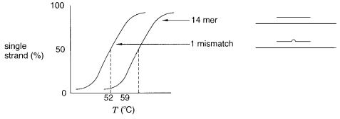
Figure 3.8 Equilibrium melting behavior of a perfectly matched oligonucleotide duplex and a duplex with a single internal mismatch.
sequence information about a larger |
DNA target. As interest in this approach becomes |
|
||||||
more developed, the necessary model |
compound data will doubtlessly be accumulated. |
|
||||||
Note that there are 12 distinct terminal mismatches, and their energetics could depend not |
|
|||||||
only on the sequence of the neighboring duplex stack but also on whether one or both |
|
|||||||
strands of |
the |
duplex are further elongated. A large number of model compounds will |
|
|||||
need to be investigated. |
|
|
|
|
|
|||
Despite the limitations and complications just described, our current ability to predict |
||||||||
the effect of a mismatch on hybridization is quite good. A typical example is shown in |
|
|||||||
Figure 3.8. Note |
that the |
melting |
transitions of oligonucleotide |
duplexes with 8 or more |
||||
base pairs |
are quite |
sharp. This reflects the large |
and |
0 |
of the |
|||
the all-or-Hnone 'snature |
||||||||
|
|
|
|
|
|
|
s |
|
reaction. The key practical concern is finding a temperature where there is good discrimi- |
|
|||||||
nation between the amount of perfect duplex formed and the amount of mismatched du- |
|
|||||||
plex. The results shown in Figure 3.8 indicate that a single internal mismatch in a 14-mer |
||||||||
leads to a 7°C decrease in |
T m . Because of |
the sharpness of the melting |
transitions, this |
|||||
can easily be translated into a discrimination of about a factor of ten in amount of duplex |
|
|||||||
present. |
|
|
|
|
|
|
|
|
KINETICS OF THE MELTING OF SHORT DUPLEXES |
|
|
||||||
The major issue we want to address here is whether, by kinetic studies of duplex dissocia- |
|
|||||||
tion, one can achieve a comparable or greater discrimination between the stability of dif- |
|
|||||||
ferent duplexes than by equilibrium melting experiments. In practice, equilibrium melting |
|
|||||||
experiments |
are |
technically |
difficult |
because one must discriminate between free and |
|
|||
bound probe or target. If the analysis is done spectroscopically, it can be done in homoge- |
|
|||||||
neous solution, but this usually requires large amounts of sample. If it is done with a ra- |
||||||||
dioisotopic tag (or a fluorescent label that shows no marked change on duplex formation), |
|
|||||||
it is usually done by physical isolation of the duplex. This assumes that the rate of duplex |
|
|||||||
dissociation is slow compared with the rate of physical separation, a constraint that usu- |
|
|||||||
ally can be met. |
|
|
|
|
|
|
|
|
In typical hybridization formats a complex is formed between probe and target, and |
||||||||
then the immobilized complex is washed to remove excess |
unbound |
probe (Fig. 3.9). |
|
|||||

78 ANALYSIS OF DNA SEQUENCES BY HYBRIDIZATION
Figure 3.9 Schematic illustration of the sort of experiment used to measure the kinetics of duplex melting.
The complex is stored under conditions where little further dissociation occurs, and af- |
|
|||||
terward |
the amount of |
probe |
bound to the target is measured. A variation on this theme |
|
||
is to allow the complex to |
dissociate for a fixed time period and then to measure the |
|
||||
amount of probe remaining bound. It turns out that this procedure gives results very sim- |
|
|||||
ilar to equilibrium duplex formation. The reason is that the temperature dependence for |
|
|||||
the reaction between two long single strands to form a duplex is very slight. The activa- |
|
|||||
tion energy for this reaction has been estimated to be only about 4 kcal/mol. Figure 3.10 |
|
|||||
shows |
a |
hypothetical |
reaction profile for interconversion between duplex and single |
|
||
strands. If we assume that the forward and reverse reaction pathways are the same, then |
|
|||||
the |
activation energy |
for |
the |
dissociation of the double strand will be just |
H 4 |
|
kcal/mol. Since |
H |
is much larger than 4 kcal/mol for most duplexes, the temperature |
|
|||
dependence of the reaction kinetics will mirror the equilibrium melting of the duplex. |
|
|||||
Figure 3.10 Thermodynamic reaction profile for oligonucleotide melting. Shown is the enthalpy,
H, as a function of strand separation.
It is simple to estimate the effect of temperature on the dissociation rate. At |
T m we ex- |
||||||
pect an equation of the form |
|
|
|
|
|
|
|
km |
A exp |
|
|
[ H |
4] |
||
|
RT |
m |
|
||||
|
|
|
|||||
|
|
|
|
|
|
|
|
KINETICS OF MELTING OF LONG DNA |
79 |
|||||||||
to apply, where |
A is a constant, and the |
exponential term reflects the number of duplexes |
|
|||||||||||||||
that have enough energy to exceed the activation energy. At any other temperature, |
|
|
|
|
|
|
|
|
T d , |
|||||||||
|
|
kd |
A exp |
|
|
[ H |
4] |
|
|
|
|
|||||||
|
|
|
RT |
d |
|
|
|
|
|
|
|
|||||||
|
|
|
|
|
|
|
|
|
|
|
|
|
|
|||||
The rate constants |
km and kd are |
for duplex melting |
at temperatures |
|
|
|
|
T m and |
T d , respec- |
|||||||||
tively. We define the time of half release at |
|
|
|
T |
d |
to be |
twash |
|
, and the time of half release at |
T m |
||||||||
to be t1/2 . Then simple algebraic manipulation of the above equations yields |
|
|
|
|
|
|
|
|
|
|||||||||
|
ln |
t |
|
|
( H 4)(1T/ |
d |
1 / T |
m |
) |
|
||||||||
|
wash |
|
|
|
|
|
|
|
|
|
|
|
|
|
||||
|
t1/2 |
|
|
|
|
|
R |
|
|
|
|
|
|
|
|
|
||
This expression allows us to calculate kinetic results for particular duplexes once measurements are made at any particular temperature.
KINETICS OF MELTING OF LONG DNA |
|
|
|
|
|
|
|
|||
The kinetic behavior of the melting of long DNA is very different from that of short |
|
|||||||||
duplexes in several respects. Melting near |
|
|
T m |
cannot |
normally be considered |
an all-or- |
||||
none reaction. Melting experiments at temperatures far above |
|
|
|
|
T m |
reveal an interesting |
||||
complication. The base pairs break rapidly, and if the |
sample |
is immediately |
returned |
|
||||||
to temperatures below |
T m , |
they |
reform |
again. |
However, if |
|
a sufficient time at high |
|||
temperature is allowed to elapse, now the renaturation rate |
can be many orders of |
|
||||||||
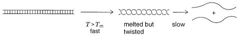
magnitude slower. What is happening is shown schematically in Figure 3.11. Once the |
|
|||||||||
DNA base pairs are broken, the two single strands are |
still twisted around |
each |
other. |
|
||||||
The twist represented by each turn of the double helix must still be unwound. As the |
|
|||||||||
untwisting begins, the process greatly slows because the coiled single strands must ro- |
|
|||||||||
tate around each other. Experiments show that the untwisting time scales as the square |
|
|||||||||
of the length of the DNA. For |
molecules |
10 kb |
or longer, these unwinding |
times |
can |
|
||||
be very long. This is probably one of the reasons why people have trouble performing |
|
|||||||||
conventional polymerase chain reaction (PCR) |
amplifications |
on |
high |
molecular |
|
|||||
weight DNA samples. The usual PCR protocols allow only 30 to 60 seconds for DNA |
|
|
||||||||
melting (as discussed in the next chapter.) This is far too short for strand untwisting of |
|
|||||||||
large DNAs. |
|
|
|
|
|
|
|
|
|
|
Figure 3.11 Kinetic steps in the melting of very high molecular weight DNA.
80 |
ANALYSIS OF DNA SEQUENCES BY HYBRIDIZATION |
|
|
KINETICS OF DOUBLE-STRAND FORMATION |
|
||
The kinetics of renaturation of short duplexes are simple and straightforward. The reac- |
|
||
tion is essentially all or none; nucleation of |
the duplex is the rate-limiting step, and |
it |
|
comes about by intermolecular collision of the separated strands. Duplex renaturation ki- |
|
||
netic measurements can be carried out at any temperature sufficiently below the melting |
|
||
temperature so that the reverse process, melting, does not interfere. The situation is much |
|
||
more complicated when longer DNAs are considered. This is illustrated in Figure 3.12 |
a, |
||
where the absorbance increase upon melting is used to measure the relative amounts of |
|
||
singleand double-stranded structures. If a melted sample, once the strands have physi- |
|
||
cally unwound, is slowly cooled, full recovery of the original duplex can be achieved. |
|
||
However, |
depending on the sample, the rate of |
duplex formation can be astoundingly |
|
slow, as we will see. If the melted sample is cooled too rapidly, the renaturation is not |
|||
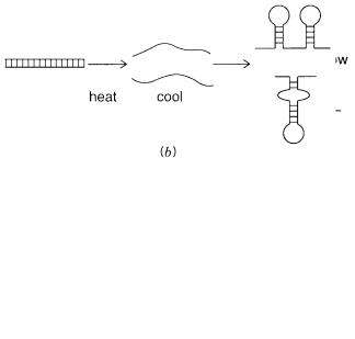
complete. In fact, as shown in Figure 3.12 |
b, true renaturation has |
not really occurred at |
|
all. Instead, the separated single strands start to fold on themselves to make hairpin duplexes, analogous to the secondary structures seen in RNA. If the temperature falls too rapidly, these structures become stable; they are kinetically trapped and, effectively, can never dissociate to allow formation of the more stable perfect double-stranded duplex.
To achieve effective duplex renaturation, one needs to hold the sample at a temperature where true duplex formation is favored at the expense of hairpin structures so that these rapidly melt, and the unfolded strands are free to continue to search for their correct partners. Alternatively, hairpin formation is kept sufficiently low so that there remains a sufficiently unhindered DNA sequence to allow nucleation of complexes with the correct partners.
Figure 3.12 |
Melting and renaturation behavior of DNA as a function of the rate |
of cooling. |
(a) |
Fraction of initial base pairing as a function of temperature. |
(b)Molecular structures |
in DNA after |
|
rapid heating and cooling. |
|
|
|

|
|
|
|
|
|
|
|
|
|
|
|
KINETICS OF DOUBLE-STRAND FORMATION |
81 |
|||||||||||||
In practice, renaturations are carried out most successfully when the renaturation tem- |
|
|
|
|
||||||||||||||||||||||
perature is ( |
T m 25)°C. In free solution the simple model, shown in Figure 3.5, is suffi- |
|
|
|||||||||||||||||||||||
cient to account for renaturation kinetics under such conditions. It is identical to the pic- |
|
|
|
|
||||||||||||||||||||||
ture used for short duplexes. The rate-limiting step is |
|
nucleation, when |
two |
strands |
|
|
|
|
||||||||||||||||||
collide in an orientation that allows the first base pair to be formed. After this, rapid du- |
|
|
|
|
||||||||||||||||||||||
plex growth occurs in both directions by a |
rapid |
zippering |
|
of the two strands together. |
|
|
|
|
||||||||||||||||||
This model predicts that the kinetics of renaturation should be a pure second-order reac- |
|
|
|
|
||||||||||||||||||||||
tion. Indeed, |
they are. If |
we call the two strands |
|
|
|
|
|
|
|
|
A |
and |
B we can |
describe |
the |
reaction |
as |
|||||||||
|
|
|
|
|
|
|
|
|
|
A |
|
B |
:AB |
|
|
|
|
|
|
|
||||||
The kinetics will be governed by a second-order rate constant |
|
|
|
|
|
|
|
|
|
|
|
k2: |
|
|
|
|||||||||||
|
|
|
|
|
|
|
d [AB ] k2[A ][B ] |
|
|
|
|
|
||||||||||||||
|
|
|
|
|
|
|
|
|
dt |
|
|
|
|
|
|
|
|
|
|
|
|
|
|
|
|
|
|
|
|
|
|
d [A ] |
d [B ] k2[A ][B ] |
|
|
|
|
||||||||||||||||
|
|
|
|
|
|
dt |
|
|
|
|
|
dt |
|
|
|
|
|
|
|
|||||||
In a typical renaturation experiment, the two strands have the same initial concentra- |
|
|
|
|
||||||||||||||||||||||
tion: [A ] [B ] C |
s |
, where |
C |
s |
is 1 the initial total concentration of DNA strands, |
|
|
|
||||||||||||||||||
o |
o |
|
|
2 |
|
|
|
|
|
|
|
|
|
|
|
|
|
|
|
|
|
|
|
|
||
|
|
|
|
|
|
|
|
|
|
|
|
|
|
|
[A ] [B |
] |
|
|
|
|
|
|
||||
|
|
|
|
|
|
|
C s |
|
|
|
o |
o |
|
|
|
|
|
|||||||||
|
|
|
|
|
|
|
|
|
|
2 |
|
|
|
|
|
|
|
|||||||||
|
|
|
|
|
|
|
|
|
|
|
|
|
|
|
|
|
|
|
|
|
|
|
|
|
||
At any subsequent time in the reaction, simple mass conservation indicates that the con- |
|
|
|
|
||||||||||||||||||||||
centrations of single strands remaining will be [ |
|
|
|
|
|
|
|
|
|
|
|
|
|
A ] [B |
] C, |
where |
C |
is the total instan- |
||||||||
taneous concentration of each strand at time |
|
|
|
|
|
|
|
|
|
|
|
|
|
|
|
t. This allows us to write the rate equation |
|
|||||||||
for the renaturation reaction as in terms of the disappearance of single strands as |
|
|
|
|
|
|||||||||||||||||||||
|
|
|
|
|
|
|
|
|
|
dC |
|
|
|
k2C 2 |
|
|
|
|
|
|
|
|||||
|
|
|
|
|
|
|
|
|
|
|
|
dt |
|
|
|
|
|
|
|
|
|
|
||||
|
|
|
|
|
|
|
|
|
|
|
|
|
|
|
|
|
|
|
|
|
|
|
|
|||
We can integrate this directly from the initial concentrations to those at any time |
|
|
|
|
|
|
t, |
|||||||||||||||||||
|
|
|
|
|
|
|
|
|
|
|
|
|
|
|
|
|
|
|
t |
|
|
|
|
|
|
|
|
|
|
|
|
|
|
|
dC |
|
k2dt |
|
|
|
|
|
|||||||||||
|
|
|
|
|
|
C 2 |
|
|
|
|
|
|||||||||||||||
|
|
|
|
|
|
|
|
|
|
|
|
|
|
|
|
|
|
0 |
|
|
|
|
|
|
|
|
which becomes |
|
|
|
|
|
|
|
|
|
|
|
|
|
|
|
|
|
|
|
|
|
|
|
|
|
|
|
|
|
|
|
|
1 |
|
|
1 |
k2t |
|
|
|
|
|
|||||||||||
|
|
|
|
|
|
|
|
|
C |
|
|
|
|
|
|
|
|
|||||||||
|
|
|
|
|
|
|
|
|
|
|
|
|
|
C |
s |
|
|
|
|
|
|
|
||||
and can be rearranged to |
|
|
|
|
|
|
|
|
|
|
|
|
|
|
|
|
|
|
|
|
|
|
|
|
|
|
|
|
|
|
|
|
|
|
C s |
|
1 |
k2tC |
s |
|
|
|
|
|
|||||||||
|
|
|
|
|
|
|
|
C |
|
|
|
|
|
|
||||||||||||
|
|
|
|
|
|
|
|
|
|
|
|
|
|
|
|
|
|
|
|
|
|
|
|
|||
82 ANALYSIS OF DNA SEQUENCES BY HYBRIDIZATION
It is convenient to rearrange this further to
|
|
C |
|
fs |
|
|
1 |
|
|
|
|
|
|
C |
|
(k2tC |
s 1) |
||||||
|
|
s |
|
||||||||
where |
fs is the fraction of original single strands remaining. |
|
|
|
|
|
|
|
|||
When |
fs 0.5, we call the time of the reaction the half time, |
|
|
|
|
t1/2 . Thus |
|||||
|
k2t1/2 C |
|
s 1 |
or |
t1/2 |
|
1 |
|
|||
|
k2C s |
||||||||||
|
|
|
|
|
|
|
|
|
|||
The key result, for a second-order reaction, is that we can adjust the halftime to any value we choose by selecting an appropriate concentration.
The concentration that enters the equations just derived is the concentration of unique, complementary DNA strands. For almost all complex DNA samples, this is not a concen-
tration we can measure directly. Usually the only concentration information readily available about a DNA sample is the total concentration of nucleotides, C
by direct UV absorbance measurements or by less direct but more sensitive fluorescence
measurements on bound dyes. To convert |
C |
0 |
|
to |
C s , we have to know something about the |
||
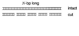
sequence of the DNA. Suppose that our DNA was the intact genome of an organism, with |
|||||||
N base pairs, as shown schematically in Figure 3.13. The concentration of each of the two |
|||||||
strands at a fixed nucleotide concentration, |
|
C |
0 , is just |
||||
C |
s |
|
|
C |
0 |
|
|
|
2N . |
||||||
|
|
|
|
|
|||
Now suppose that the genome is divided into chromosomes, or the chromosomes into unique fragments, as shown in Figure 3.13. This does not change the concentration of any of the strands of these fragments. (An important exception occurs if the genome is ran-
domly broken instead of uniquely broken; see Cantor and Schimmel, 1980.) Thus we can
write the product of |
k2, the concentration and half-time, as |
|
|
||
|
k2t1/2 C s |
|
k2t1/2 C |
0 |
1 |
|
2N |
|
|||
|
|
|
|
|
|
and this can be rearranged to
C 0 t1/2 2N
k2
Figure 3.13 Schematic illustration of intact genomic DNA, or genomic DNA digested into a set of nonoverlapping fragments.

|
|
|
|
|
|
|
|
KINETICS OF DOUBLE-STRAND FORMATION |
83 |
||||||
This key result means that the rate of genomic DNA reassembly depends linearly on the |
|
|
|
||||||||||||
genome size. Since genome sizes vary across many orders of magnitude, the resulting re- |
|
|
|
||||||||||||
naturation rates will also. Here we have profound implications for the design and execu- |
|
|
|
||||||||||||
tion of experiments that use genomic DNA. Molecular biologists have tended to lump the |
|
|
|
||||||||||||
two variables |
C 0 and |
t1/2 together, and they talk about the parameter |
C |
0 t1/2 |
as “a half cot.” |
||||||||||
We will use this term, but don’t try to sleep on it. |
|
|
|
|
|
|
|
|
|
|
|||||
Some predicted kinetic results for the renaturation of genomic DNA that illustrate the |
|
|
|||||||||||||
renaturation behavior of the different samples are shown in Figure 3.14. These results are |
|
|
|
||||||||||||
calculated |
for |
typical |
renaturation |
conditions |
with |
a |
nucleotide |
concentration |
of |
|
|
||||
1.5 10 |
4 M. Note |
that |
under |
these conditions |
a |
3-kb plasmid will renature so |
quickly |
|
|
||||||
that it is almost impossible to work with the separate strands under conditions that allow |
|
|
|
||||||||||||
renaturation. In contrast, the 3 |
10 |
9 |
bp human genome is predicted to require 58 days to |
|
|||||||||||
renature under the very same conditions. In practice, this means never; much higher con- |
|
|
|||||||||||||
centrations must be used to achieve the renaturation of total human DNA. |
|
|
|
|
|
||||||||||
The actual renaturation results seen for human DNA are very different from the simple |
|
|
|
||||||||||||
prediction we just made. The reason is a significant fraction of human DNA is highly re- |
|
|
|
||||||||||||
peated sequences. This changes the renaturation rate of these sequences. The concentra- |
|
|
|
||||||||||||
tion of strands of a sequence repeated |
|
|
m |
times in |
the genome is |
m C |
0 /2N |
. Thus this se- |
|||||||
quence will renature much faster: |
|
|
|
|
|
|
|
|
|
|
|
||||
|
|
|
|
|
|
|
|
C 0 t1/2 |
2N |
|
|
|
|
||
|
|
|
|
|
|
|
|
mk 2 |
|
|
|
||||
|
|
|
|
|
|
|
|
|
|
|
|
|
|||
The same equation also handles the case of heterogeneity in which a particular sequence |
|
|
|
||||||||||||
occurs in only a fraction of the genomic DNA under study. In this case |
|
|
|
m 1, and the re- |
|||||||||||
naturation proceeds slower than expected. Typical renaturation results for human (or any |
|
|
|
||||||||||||
mammalian) |
DNA |
are shown |
in |
Figure |
3.15. There |
are |
three |
clearly |
resolved kinetic |
|
|
||||
Figure 3.14 |
Renaturation kinetics expected for different DNA samples at a total initial nucleotide |
|
concentration of 1.5 |
10 4 M at typical salt and temperature |
conditions. The fraction of single |
strand remaining, f |
s , is plotted as a function of the log of the time, |
t. Actual experiments conform to |
expectations except for the human DNA sample. See Figure 3.15.