

Vankka J. - Digital Synthesizers and Transmitters for Software Radio (2000)(en)
.pdf80 |
Chapter 5 |
[Gol69] B. Gold, and C. M. Rader, "Digital Processing of Signals," New York: McGraw-Hill, 1969.
[Gor85] J. W. Gordon and J. O. Smith, "A Sine Generation Algorithm for VLSI Applications," in Proc. 1985 International Computer Music Conference (ICMC), Vancouver, 1985, pp. 165-168.
[Gra98] E. Grayver, and B. Daneshrad, "Direct Digital Frequency Synthesis Using a Modified CORDIC," Proc. IEEE Int. Symp. Circuits and Systems (ISCAS), Vol. 5, pp. 241–244, 1998.
[Har83] I. Hartimo, "Self-Sustained Stable Oscillations of Second Order Recursive Algorithms," in Proc. IEEE Int. Conference on Acoustics, Speech, and Signal Processing, USA, Apr. 1983, pp. 635-638.
[Kro96] B. W. Kroeger, and J. S. Baird "Numerically Controlled Oscillator with Complex Expotential Outputs Using Recursion Technique," U. S. Patent 5,517,535, May. 14, 1996.
[Pal00] K. I. Palomäki, J. Niittylahti, and V. Lehtinen, "A Pipelined Digital Frequency Synthesizer Based on Feedback," Proceedings of the 43rd IEEE Midwest Symposium on Circuits and Systems, Vol. 2, Aug. 2000 pp. 814-
817.
[Pal99] K. I. Palomäki, J. Niittylahti, and M. Renfors, "Numerical Sine and Cosine Synthesis Using a Complex Multiplier," Proceedings of the 1999 IEEE International Symposium on Circuits and Systems, Vol. 4, June 1999, pp. 356 -359.
[Pre94] L. Presti, and G. Cardamone, "A Direct Digital Frequency Synthesizer Using an IIR Filter Implemented with a DSP Microprocessor," IEEE Int. Conf. Acoustics, Speech, and Signal Processing (ICASSP), Vol. 3, pp.
201–204, 1994.
[Pro97] J. G. Proakis, and D. G. Manolakis, "Digital Signal Processing, Principles," Macmillan Publishing Company, 1998, pp. 365.
[Tur03] C. S. Turner, "Recursive Discrete-Time Sinusoidal Oscillators," IEEE Signal Processing Magazine, Vol. 20, No. 3, pp. 103–111, May 2003.

Chapter 6
6. CORDIC ALGORITHM
Algorithms used in communication technology require the computation of trigonometric functions, coordinate transformations, vector rotations, or hyperbolic rotations. The CORDIC, an acronym for COordinate Rotation DIgital Computer, algorithm offers an opportunity to calculate the desired functions in a rather simple and elegant way. The CORDIC algorithm was first introduced by Volder [Vol59]. Walter [Wal71] later developed it into a unified algorithm to compute a variety of transcendental functions. Two basic CORDIC modes leading to the computation functions exist, the rotation mode and the vectoring mode. For both modes the algorithm can be realized as an iterative sequence of additions/subtractions and shift operations, which are rotations by a fixed rotation angle, but with a variable rotation direction. Due to the simplicity of the operations involved, the CORDIC is very well suited for a VLSI realization ([Sch86], [Dur87], [Lee89], [Not88], [Bu88], [Cav88a], [Cav88b], [Lan88], [Sar98], [Kun90], [Lee92], [Hu92b], [Fre95], [Hsi95], [Phi95], [Ahn98], [Dac98], [Mad99]). It has been implemented in pocket calculators like Hewlett Packard's HP-35 [Coc92], and in arithmetic coprocessors like Intel 8087.
In this book, the interest is in the rotation mode, because the QAM modulator (our application) performs a circular rotation (see (4.10)). The basic task performed in the CORDIC algorithm is to rotate a 2 by 1 vector through an angle using a linear, circular or hyperbolic coordinate system [Wal71]. This is accomplished in the CORDIC by rotating the vector through a sequence of elementary angles whose algebraic sum approximates the desired rotation angle.
The CORDIC algorithm provides an iterative method of performing vector rotations by arbitrary angles using only shifts and adds. The algorithm is derived from the general rotation transformation. In Figure 6-1, a pair of rec-

82 Chapter 6
tangular axes is rotated clockwise through the angle Ang by the CORDIC algorithm where the coordinates of a vector transform (I Q) to (I’ Q’)
I |
I cos(Ang) + Qsin(Ang) |
|
(6.1) |
Q |
Qcos(Ang) I sin(Ang). |
|
|
which rotates a vector clockwise in a Cartesian plane through the angle Ang as shown in Figure 6-1. These equations can be rearranged so that
|
|
|
|
|
|
|
|
|
|
|
|
|
|
I' |
cos(Ang) [ |
|
|
|
|
|
|
|
|
|
] |
(6.2) |
|
|
|
|
|
|
|
|
|
|
|||||
Q |
cos(Ang) [ |
|
|
|
|
|
|
|
|
|
] |
||
|
|
|
|
|
|
|
|
|
|
||||
|
|
|
|
|
|
|
|
|
|
||||
|
|
|
|
|
|
|
|
|
|
|
|
|
|
If the rotation angles are restricted to tan(Angi) = ±2 , the multiplication by the tangent term is reduced to a simple shift operation. Arbitrary angles of rotation are obtainable by performing a series of successively smaller elementary rotations. If the decision at each iteration, i, is which direction to rotate rather than whether or not to rotate, then the term cos(Angi) becomes a constant, because cos(Angi) = cos(-Angi). The iterative rotation can now be expressed as
I |
i+1 |
K |
i |
[I |
i |
|
+ Q |
i |
|
d |
i |
|
2 i ] |
(6.3) |
|||||||||||
|
|
Ki [ |
|
|
|
|
|
|
|
|
|
|
|
|
|
|
|
|
|
|
|
] |
|||
Qi+1 |
|
|
|
|
|
|
|
|
|
|
|
|
|
|
|
|
|
|
|
|
|||||
where di = ±1 and |
|
|
|
|
|
|
|
|
|
|
|
|
|
|
|
|
|
|
|
|
|
|
|
|
|
Ki cos(tan |
1 (2 |
|
i )) |
|
1 / |
|
|
|
|
(1 + 2 2i ) |
(6.4) |
||||||||||||||
|
|
|
|
|
|
|
|
|
|
|
|
|
|
|
|
|
|
|
|
|
|
|
|
|
|
Removing the scale constant from the iterative equations yields a shift-add algorithm for the vector rotation. The product of the Ki ’s approaches 0.6073 as the number of iterations goes to infinity. The exact gain depends on the number of iterations, and obeys the relation
|
|
N |
1 |
|
G |
N |
= ∏ |
(1 + 2 2i ) |
(6.5) |
|
i 0 |
|
||
|
|
|
||
|
|
|
|
|
Q


 ANG
ANG
Q' 


II'
Figure 6-1 . Vector rotation.

CORDIC Algorithm |
83 |
The CORDIC rotation algorithm has a gain, GN, of approximately 1.647 as the number of iterations goes to infinity.
If both vector component inputs are set to the full scale simultaneously, the magnitude of the resultant vector is 1.414 times the full scale. This, combined with the CORDIC gain, yields a maximum output of 2.33 times the full-scale input.
The angle of a composite rotation is uniquely defined by the sequence of the directions of the elementary rotations. This sequence can be represented by a decision vector. The set of all possible decision vectors is an angular measurement system based on binary arctangents. Conversions between this angular system and others can be accomplished using an additional adder/subtractor that accumulates the elementary rotation angles at each iteration. The angle computation block adds a third equation to the CORDIC algorithm
zi+1 zi di tan 1 (2 i ) |
(6.6) |
|
|
The CORDIC algorithm can be operated in one of two modes. The first one, called rotation by Volder [Vol59], rotates the input vector by a specified angle (given as an argument). The second mode, called vectoring, rotates the input vector to the I axis while recording the angle required to make that rotation. The CORDIC circular rotator operates in the rotation mode. In this mode, the angle computation block is initialized with the desired rotation angle. The rotation decision at each iteration is made in order to decrease the magnitude of the residual angle in the angle computation block. The decision at each iteration is therefore based on the sign of the residual angle after each step. The CORDIC equations for the rotation mode are
Ii+1 |
Ii |
+ Qi di 2 i |
|
Qi+1 |
Qi |
Ii di 2 i |
(6.7) |
zi+1 |
zi |
di tan 1 (2 i ), |
|
where di = -1 if zi < 0, and +1 otherwise, so that z is iterated to zero. These equations provide the following result, after n iterations
|
|
|
|
|
|
|
|
|
|
|
|
|
|
|
|
|
|
|
|
|
|||
In |
Gn |
[ |
|
|
|
|
|
|
|
|
|
|
|
|
|
|
|
|
|
] |
|||
|
|
|
|
|
|
|
|
|
|
|
|
|
|
|
|
|
|
||||||
[ |
|
|
|
|
|
|
|
|
|
|
|
|
|
|
|
|
|
|
] |
||||
Qn |
Gn |
|
|
|
|
|
|
|
|
|
|
|
|
|
|
|
|
|
|
||||
|
|
|
|
|
|
|
|
|
|
|
|
|
|
|
|
|
|
||||||
|
|
|
|
|
|
|
|
|
|
|
|
|
|
|
|
|
|
||||||
|
|
(6.8) |
|||||||||||||||||||||
|
|
n 1 |
|
|
|||||||||||||||||||
G |
n |
∏ |
|
|
1 + 2 2i |
||||||||||||||||||
|
i 0 |
|
|
|
|
|
|
|
|
|
|
|
|
|
|
|
|
|
|
|
|
|
|
|
|
|
|
|
|
|
|
|
|
|
|
|
|
|
|
|
|
|
|
|
|
|
|
AAng zn
where A is the rotated angle

84 |
|
|
|
|
|
|
|
|
|
|
|
|
|
|
|
|
|
Chapter 6 |
|
|
|
|
|
|
|
|
|
|
|
|
|
|
|
|
|
|
|
|
|
|
|
n |
1 |
|
|
|
|
|
|
|
|
|
|
|
|
|
|
|
|
|
¦ |
|
|
|
|
|
|
|
|
|
|
|
). |
(6.9) |
|
|
|
|
|
|
|
|
|
|
|
|
|
|
|
|
|
|||
|
|
|
|
i |
0 |
|
|
|
|
|
|
|
|
|
|
|
|
|
|
|
|
|
|
|
|
|
|
|
|
|
|
|
|
|
|
|
|
The CORDIC rotation algorithm as stated is limited to rotation angles between - /2 and /2, because of the use of 20 for the tangent in the first iteration. For composite rotation angles larger than /2, an initializing rotation is required. For example, if it is desired to perform rotations with rotation angles between - and , it is necessary to make an initial rotation of ± /2
I0 |
d Qin , |
|
|||
Q0 |
|
|
d Iin |
(6.10) |
|
z |
0 |
z |
in |
d 2 tan−1 |
(20 ), |
|
|
|
|
||
|
|
|
|
|
|
where d = -1 if zin < 0, and +1 otherwise.
6.1 Scaling of In and Qn
The results from the CORDIC operation have to be corrected because of the inherent magnitude expansion in the circular mode. This increases the latency and requires a lot of hardware. Many articles have dealt with this problem and have suggested different methods to reduce the cost of the scaling. Timmermann et al. compares the different approaches in [Tim91].
Each iteration of the CORDIC algorithm extends the vector [Ii Qi] in the rotational mode. Because of this, the resulting vector [In Qn] has to be scaled with the scaling factor Gn given in (6.5). The correction due to the scaling factor can be performed in three different ways:
1.Post-multiplying the result In, Qn or pre-multiplying the input I0 Q0 with 1/Gn. This is the straightforward way to compensate for the scaling factor; it increases the latency with one multiplication.
2.Separate scaling iterations can be included in the CORDIC algorithm, or CORDIC iterations can be repeated, such that the scaling factor becomes a power of two, thus reducing the final scaling operation to a shift operation [Ahm82], [Hav80].
3.The CORDIC iterations can be merged with the scaling factor compensation (as described in [Bu88]).
The conclusion in [Tim91] is that the third type of scaling tends to increase the overall latency. Therefore, to minimize the latency, the normal iterations and the scaling should be separated.
In our design, the scaling factor is constant because the number of the iterations is constant. The scaling factor is simply factored into an aggregate

CORDIC Algorithm |
85 |
processing gain attributed to the filter chain in the QAM modulator (see Figure 16-6).
6.2 Quantization Errors in CORDIC Algorithm
Hu [Hu92a] provided an accurate description of the errors encountered in all modes of the CORDIC operation. In [Hu92a], two major sources of error are identified: the (angle) approximation error and the rounding error. The first type of error is due to the quantized representation of a CORDIC rotation angle by a finite number of elementary angles. The second one is due to the finite precision arithmetic used in a practical implementation. However, the bound for the approximation error has been set without taking into account the effects of the quantization of the angles (the inverse tangents). In [Kot93], the study of the numerical accuracy in the CORDIC includes the accuracy problem with the inverse tangent calculations. The error analysis in [Hu92a] and [Kot93] is based on the assumption that an error reaches its maximum value at each quantization step. This gives quite pessimistic results especially in QAM modulator applications, where the I/Q inputs are random signals.
6.2.1 Approximation Error
The equations (6.7) can be rewritten as
|
|
|
|
|
|
|
vi+1 |
|
pi vi |
|
|
|
|
|
|
|
(6.11) |
|
where vi = [Ii Qi]T is the rotation vector at the ith iteration, and |
|
|
||||||||||||||||
|
|
ª |
1 |
d |
i |
2 |
i º |
|
|
2i |
ª |
cosa |
i |
d |
i |
sina |
i |
º |
p |
|
= |
|
|
|
= |
1 |
+ 2 |
|
|
|
|
(6.12) |
|||||
i |
di 2 i |
|
|
|
|
¬ |
|
|
|
|
|
|
||||||
|
¬ |
|
|
1 |
¼ |
|
|
|
di sinai |
|
cosai |
|
¼ |
|||||
|
|
|
|
|
|
|
|
|
||||||||||
|
|
|
|
|
|
|
|
|
|
|
|
|
|
|
|
|
|
|
is an unnormalized rotation matrix. The magnitude of the elementary angle rotated in the ith iteration is ai = tan-1 (2 i).
In the CORDIC algorithm, each rotation angle A is represented by a restricted linear combination of the n elementary angles ai (n is the number of iterations), as follows:
n |
1 |
|
Ang ¦di ai + zn A + zn |
(6.13) |
|
i |
0 |
|
where zn is the error due to this angle quantization. The CORDIC computation error in vn due to the presence of "zn" is defined as the approximation error. In the following derivations, infinite precision arithmetic will be applied in order to suppress the effect due to the rounding error.

86 |
Chapter 6 |
Conventionally, in the CORDIC algorithm, two convergence conditions will be set [Hu92a]. The first condition states that the rotation angle must be bounded
|
|
n 1 |
|
A |
|
≤ Σ ai ≡ A |
(6.14) |
|
|||
|
|
i 0 |
|
The second condition is set to ensure that if the rotation angle A satisfies (6.14), its angle approximation error will be bounded by the smallest elementary rotation angle an-1 . That is,
|
zn |
|
≤ an 1 |
(6.15) |
|
|
|||
|
|
|||
To satisfy this condition, the elementary angle sequence (ai |
i = 0 to i n |
|||
1) must be chosen so that [Wal71] |
|
|
||
|
n 1 |
|
|
|
ai - |
Σ |
a j ≤ an 1 |
(6.16) |
|
|
|
|||
j i+1
Based on the above result, it is quite obvious, that in order to minimize the approximation error, the smallest elementary rotation angle an-1 must be made small. This can be achieved by increasing the number of the CORDIC iterations.
6.2.2 Rounding Error of Inverse Tangents
If the numerically controlled oscillator (NCO) output in Figure 16-6 has a long period (from (4.4)), then the approximation errors are uncorrelated and uniformly distributed within each quantization step
− a |
|
|
|
≤ z |
≤ |
a |
|
(6.17) |
||||
n |
|
|
n |
|
|
|
n |
|
||||
The quantization of the angles is defined as |
|
|||||||||||
|
|
|
|
|
|
|
|
|
|
], |
(6.18) |
|
|
|
|
|
|
|
|
|
|
||||
|
|
|
||||||||||
where Q[.] denotes the quantization operator and the rounding error is |
|
|||||||||||
|
|
|
2π |
≤ ei |
≤ 2π |
(6.19) |
||||||
|
2ba+1 |
|
|
2ba+1 |
|
|||||||
for a fixed-point angle computation data path with ba bits, which is assumed to be greater than the number of iteration stages (n). This is a reasonable assumption because the size of the residual angle becomes smaller in the successive iteration stages, approximately by one bit after each iteration.

CORDIC Algorithm |
87 |
6.2.3 Rounding Error of In and Qn
The rounding error of zn is quite straightforward as it involves only the inner product operation. Hence, the focus will be on the rounding error in In and
Qn . The quantization of the error vi = [Ii Qi |
]T is defined as |
||||||
ª Ii º |
ªQ[ |
|
|
|
]º |
||
|
|||||||
ei |
|
|
(6.20) |
||||
¬Qi ¼ |
¬Q[ |
|
|
|
|
|
]¼ |
|
|
|
|||||
|
|
|
|
||||
|
|
|
|
||||
where ei = [eiI eiQ]T is an error vector due to rounding. For the fixed-point arithmetic, the absolute rounding error will be bounded by
eiI ≤ 2 bb |
eiQ ≤ 2 bb |
(6.21) |
2 |
2 |
|
where bb is the number of fractional bits in the angle rotation data path. The variance of the error is (assuming that the error is a white noise process and probability distribution of the error sample values is uniform over the range of the quantization error)
δ I2 δ Q2 |
2 |
2bb |
|
|
|
(6.22) |
|
|
12 |
||
|
|
|
|
The variance of the rounding error of Ii and Qi is
δ IQ2 δ I2 |
+ δ Q2 |
2 |
2bb |
|
|
|
(6.23) |
||
|
6 |
|||
|
|
|
|
|
In each CORDIC iteration, the rounding error consists of two components: the rounding error propagated from the previous iterations and the rounding error introduced in the present iteration. The variance due to the rounding error of In and Qn at the CORDIC rotator output is therefore
|
|
|
n 1 |
n 1 |
|
|
δ t2ot2 δ I2Q 1 |
+ |
Σ |
∏ |
Ki2 |
(6.24) |
|
|
|
|||||
|
|
|
j 0 |
i j |
|
|
where Ki2 is (1 + 2-2i) from equation (6.12).
6.3 Redundant Implementations of CORDIC Rotator
The computation time and the achievable throughput of CORDIC processors using conventional arithmetic are determined by the carry propagation involved with the additions/subtractions, since the direction of the CORDIC microrotation is steered by the sign of the previous iteration results. This sign is not known prior to the computation of the MSB. The use of redundant arithmetic is well known to speed up additions/subtractions, because a carry-
88 |
Chapter 6 |
free or limited carry-propagation operation becomes possible. However, the application of redundant arithmetic in the CORDIC is not straightforward, because a complete word level carry-propagation is still required in order to determine the sign of a redundant number (this also holds for generalized signed digit numbers as described in [Par93]).
In order to overcome this problem, several authors have proposed techniques for estimating the sign of the redundant intermediate results from a number of MSDs (most significant digits) ([Erc90], [Erc88], [Tak87]). If the sign, and therefore the rotation direction, cannot be estimated reliably from the MSDs, no microrotation occurs at all. However, the scaling factor involved in the CORDIC algorithm depends on the actual rotations. Therefore, here, the scaling factor is variable, and has to be calculated in parallel to the usual CORDIC iteration. Additionally, a division by the variable scaling factor has to be implemented following the CORDIC iteration.
A number of publications dealing with constant scale factor redundant (CSFR) CORDIC implementations of the rotation mode ([Erc90], [Erc88], [Tak87], [Kun90], [Nol91], [Tak91], [Lin90], [Nol90], [Yos89]) describe sign estimation techniques, where every iteration is reactually performed, in order to overcome this problem. However, either a considerable increase (about 50 per cent) in the complexity of the iterations (double rotation method [Tak91]) or a 50 percent increase in the number of iterations (correcting iteration method [Tak91], [Nol90], [Kun90], [Nol91]) occurs.
In [Dup93], a different CSFR algorithm is proposed for the rotation mode. Using this "branching CORDIC", two iterations are performed in parallel if the sign cannot be estimated reliably, each assuming one of the possible choices for the rotation direction. It is shown in [Dup93] that, at most, two parallel branches can occur. However, this is equivalent to an almost twofold effort in terms of implementation complexity of the CORDIC rotation engine. In contrast to the above mentioned approaches, in [Daw96], transformations of the usual CORDIC iteration are developed, resulting in a constant scale factor redundant implementation without additional or branching iterations. It is shown in [Daw96] that this "Differential CORDIC (DCORDIC)" method compares favorably to the sign estimation methods.
However, the architecture described in Section 16.5 does not use any of these techniques. The adder/subtractors used in the CORDIC rotator unit allow the operation frequency to be reached with carry-ripple arithmetic, and therefore the problem of sign estimation is avoided.
6.4 Hybrid CORDIC
Ahmed has developed a hybrid approach to elementary function generation that combines memory, multipliers and the CORDIC [Ahm82], [Ahm89].
CORDIC Algorithm |
89 |
The vector rotation by angle (Ang) could be partitioned into two parts, a coarse rotation stage and fine rotation stage [Ahm89]. The basic principle is general, although Ahmed has restricted his attenuation to the CORDIC rotation algorithm in [Ahm89]. Similar results were published in [Tim89], [Hwa03] but the effect on the vectoring mode were considered. Wang generalized Ahmed’s work and presented two Hybrid CORDIC algorithms: Mixed Hybrid algorithm and Partioned-Hybrid algorithm based on [Wan97]. The hybrid CORDIC algorithms offer a considerable latency time reduction and chip area savings when compared with the original CORDIC algorithm [Wan97].
6.4.1 Mixed-Hybrid CORDIC Algorithm
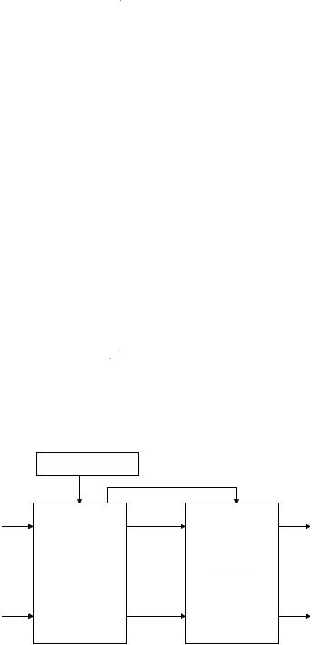
The architectural approach for the case of the Mixed-Hybrid CORDIC algorithm is given in Figure 6-2. The CORDIC iterations related to the coarse part are performed as in the conventional CORDIC algorithm. In order to avoid errors, each rotation direction can be evaluated only after the previous iteration has been completed. The iterations related to the fine part can be simplified [Ahm89], [Tim89]. Applying the Taylor series expansions to the z data path in (6.6), and taking only the first terms, the z data path becomes
z |
i+1 |
z |
i |
− d |
i |
2 i |
(6.25) |
|
|
|
|
|
In [Wan97], it has been showed that the rotation directions for approximately 2/3 of the iterations (N) can be derived using (6.25) in the rotation mode. The error is negligible in finite length arithmetic [Wan97]. All rotation directions associated with such iterations are available in parallel, since each of them is given by the corresponding bit of the residue rotation angle (1 and 0 identify positive and negative rotation, respectively). It is worthwhile noting that application of the CORDIC iterations related to the most
Ang
|
|
z0 |
zn |
|||
|
|
|
|
|
||
I0 |
|
|
In |
|
|
IN |
|
|
|
|
|||
|
|
COARSE |
|
|
FINE |
|
|
ROTATOR |
|
|
ROTATOR |
|
|
Q0 |
|
|
Qn |
|
|
QN |
|
|
|
|
|
|
|
Figure 6-2. The architecture for Mixed-Hybrid CORDIC algorithms.