Vankka J. - Digital Synthesizers and Transmitters for Software Radio (2000)(en)

MUX

-h4k+2

Q

-h4k+3

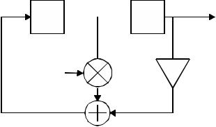
Figure 4-6 Simplified digital modulator.

enables the transmission of signals having different symbol rates.

REFERENCES

[Ahm89] H. M. Ahmed, "Efficient Elementary Function Generation with Multipliers," in Proc. 9th Symposium on Computer Arithmetic, Santa Monica, CA, USA, Sept. 1989, pp. 52-59.

[Bra81] A. L. Bramble, "Direct Digital Frequency Synthesis," in Proc. 35th Annu. Frequency Contr. Symp., USERACOM (Ft. Monmouth, NJ), May 1981, pp. 406-414.

[Cro83] R. E. Crochiere, and L. R. Rabiner, "Multirate Digital Signal Processing," Englewood Cliffs, NJ: Prentice-Hall, 1983.

[Cur01] F. Curticãpean, and J. Niittylahti, "An Improved Digital Quadrature Frequency Down-Converter Architecture," Asilomar Conf. on Signals, Syst. and Comput., Nov. 2001, pp. II-1318-1321.

[Dar70] S. Darlington, "On Digital Single-Sideband Modulators," IEEE Trans. Circuit Theory, Vol. 17, No. 3, pp. 409-414, Aug. 1970.

[Dut78] D. L. Duttweiler, and D. G. Messerschmitt, "Analysis of Digitally Generated Sinusoids with Application to A/D and D/A Converter Testing," IEEE Trans. on Commun., Vol. COM-26, pp. 669-675, May 1978.

[Gol96] B. G. Goldberg, "Digital Techniques in Frequency Synthesis," McGraw-Hill, 1996.

[Gor75] J. Gorski-Popiel, "Frequency-Synthesis: Techniques and Applications," IEEE Press, New York, USA, 1975.

[Hog81] E. B. Hogenauer, "An Economical Class of Digital Filters for Decimation and Interpolation," IEEE Trans. Acoust., Speech, Signal Process., Vol. ASSP-29, No. 2, pp. 155-162, Apr. 1981.

we obtain from (5.3) a discrete-time sinusoidal function as the output signal:

It has complex-conjugate poles at p = exp(±jθout), and a unit sample response y(n) A cos(nθ out ), n ≥ 0 (5.8)

Thus the impulse response of the second-order system with complexconjugate poles on the unit circle is a sinusoidal waveform.

Thus, any real-valued sinusoidal oscillator signal can be generated by the second-order structure shown in Figure 5.1.

In fact, the difference equation in (5.1) can be obtained directly from the trigonometric identity

A cos(θ out (n + 2)) A 2cos(θ out )cos(θ out (n + 1)) A cos(θ out n), (5.12) where, by definition, x2(n + 2) = Acos(cosθout(n + 2)).

The output sequence y(n) of the ideal oscillator is the sampled version of a pure sine wave. The angle θout represented by the oscillator coefficient is given by

where f ut is the desired output frequency. In an actual implementation, the multiplier coefficient 2 cosθout is assumed to have b + 2 bits. In particular, 1

z-1 z-1

y(n)

Figure 5.1. Recursive digital oscillator structure.

bit is for the sign, 1 bit for the integer part and b bits for the remaining fractional part in the fixed-point number representation. Then the largest value of the coefficient 2 cosθout that can be represented is (2 – 2 b). This value of the coefficient gives the smallest value of θmin that can be implemented by the direct form digital oscillator using b bits

Therefore, the smallest frequency that the oscillator can generate is

where f is the sampling frequency. It should be emphasized that the frequency resolution of the direct-form oscillator is a function of the wordlength of the multiplier coefficient. Therefore, to increase the frequency resolution, the wordlength of the multiplier coefficient must be increased. Because the poles generated by a quantized coefficient (2 cosθout) are not uniformly distributed on the unit circle, the distance between two adjacent generated frequencies varies (the distance decreases as the generated frequency increases). The inability of the direct form digital oscillator to generate equally spaced frequencies is a disadvantage from the point of view of a communication system. A modified direct-form digital oscillator capable of generating almost equally spaced frequencies has been proposed in [Ali97]. However, it comes at a higher hardware cost as the solution in [Ali97] requires one additional multiplier and two integrators.

Every time when the frequency is changed, a new set of parameters have to be computed. For the direct-form digital oscillator it is rather difficult to keep the phase continuous when the frequency is changed. This is a disadvantage if compared with the DDS (Figure 4-1).

In this digital oscillator, besides the zero-input response y(n) of the sec- ond-order system we get a zero-state response yerr(n) due to the random sequence e2(n) acting as an input signal. From (5.1) we obtain

with Yideal (z) derived from (5.7). The z transform of the output error yerr(n) is given by

with E2(z) being the z transform of the quantization error signal e2(n). Transforming Yerr(z) back into the time domain results in an output error sequence

n

yerr (n) θ1 ¦ e2 (k) sin(θout (n k + 1)) for n ≥ 2 (5.19)

sin out k 2

where e2(0) and e2(1) are assumed to be zero. Equation (5.19) shows that the output error is inversely proportional to sin(θout), thus the output error increases with the decreasing digital oscillator frequency. The accumulation of the quantization errors degrades the spectral purity of the generated wave and can produce computation overflows. Such computation overflows can easily make the oscillator unstable.

The output quantization error can be reduced by an appropriate error feedback [Abu86b]. In addition to the error feedback, a periodic oscillator reset could be applied. In order to eliminate an infinite accumulation of errors, the direct-form oscillator could be reset to its initial states after N samples (K cycles) if the normalized frequency θout/2 equals the rational number K/ N [Fur75]. This method is not effective for a large N, because the accumulated error will also be large. As a result, the signal spectrum will be degraded. Therefore, it is possible to reset the oscillator many times over one period (N) in [Fur75].

5.2 Coupled-Form Complex Oscillator

The coupled-form digital oscillator generates simultaneously sine and the cosine waves (Asinθoutn and Acosθoutn) [Gol69], [Gor85], [Fli92], [Kro96], [Pro97], [Gra98], [Pal99], [Pal00], [Tur03] and can be obtained from the trigonometric formulae

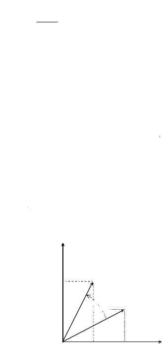
x2(n+1)

θout

x2(n)

x1(n+1) x1(n)

Figure 5.2. Vector rotation

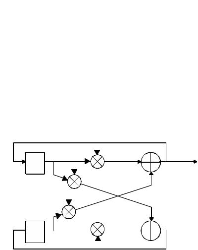
that perform a general rotational transform anti-clockwise with angle θout the coordinates of a vector in Figure 5.2 transform from (x1 (n), x2(n)) to (x1 (n+1), x2(n+1)). The structure for the realization of the coupled-form oscillator is illustrated in Figure 5.3. This is a two-output system which is not driven by any input, but which requires the initial conditions x1 (0) = Acos(θout) and x2(0) = Asin(θout) in order to begin its self-sustaining oscillations.

Obviously, the total hardware cost of the coupled-form digital oscillator (Figure 5.3) is significantly higher than the cost of a direct-form oscillator (Figure 5.1). The coupled-form complex oscillator in Figure 5.3 could be implemented by a complex multiplier [Kro96], [Gra98], [Pal99], [Pal00]. The drawback of this method is low maximum clock frequency, which is limited by the speed of the complex multiplier. Due to the recursion, regular pipelining cannot be utilized [Pal00]. The design in [Gra98] uses CORDIC algorithm to compute the initial values.

Changing the frequency of the sinusoids generated by the coupled-form oscillator is simpler than in the case of the direct-form oscillator, because

cosθout

Acos((n+1)θout)

z-1 sinθout

-sinθout

Asin((n+1)θout)

z-1

cosθout

Figure 5.3. Coupled-form complex oscillator.

tive amount to a lower value, both would be raised, in one iteration cycle, to the value they would have had if no noise were present. If, however, x2(n) had drifted up and x1 (n) down so that the sum of the squares were satisfied (5.25), then (5.27) would have no effect. Thus the drifts of phase are not compensated by (5.27). In [Fli92], the amplitude gain is controlled by changing the oscillator coefficients. If f( n) is larger than one, then the coefficientset generating poles outside the unit circle are utilized. If f( n) is smaller than one, then the coefficient-set generating poles inside the unit circle are used for computing the next sample. By these means, the amplitude of the generated waves is kept within given limits. Other amplitude correction methods are presented in [Gra98], [Pal99], [Pal00]. In these methods, the feedback signal is saturated if overflows or underflows occur. The most efficient method of eliminating the infinite accumulation of errors of the coupledform complex oscillator is to reset its initial states after N samples (K cycles) if the normalized frequency θout/2 equals the rational number K/ N

An increase in the frequency resolution requires that the word length of the whole complex oscillator is widened; however, in the case of the conventional direct digital synthesizer, it is only necessary to increase the phase accumulator word length (see (4.2)).

REFERENCES

[Abu86a] A. I. Abu-El-Haija, and M. M. Al-Ibrahim, "Digital Oscillator Having Low Sensitivity and Roundoff Errors," IEEE Trans. on Aerospace and Electronic Systems, Vol. AES-22, No. 1, pp. 23-32, Jan. 1986.

[Abu86b] A. I. Abu-El-Haija, and M. M. Al-Ibrahim, "Improving Performance of Digital Sinusoidal Oscillators by Means of Error-Feedback Circuits," IEEE Trans. Circuits Syst., Vol. CAS-33, pp. 373-380, Apr. 1986.

[Ali01] M. M. Al-Ibrahim, "A Multifrequency Range Digital Sinusoidal Oscillator with High Resolution and Uniform Frequency Spacing," IEEE Trans. on Circuits and Systems II, Vol. 48, No. 9, pp. 872-876, Sept. 2001.

[Ali97] M. M. Al-Ibrahim and A. M. Al-Khateeb, "Digital Sinusoidal Oscillator with Low and Uniform Frequency Spacing," IEE Proceedings on Circuits, Devices and Systems, Vol. 144, No. 3, pp. 185-189, June. 1997.

[Asg93] S. M. Asghar, and A. R. Linz, "Frequency Controlled Recursive Oscillator Having Sinusoidal Output," U. S. Patent 5,204,624, Apr. 20, 1993. [Fli92] N. J. Fliege, and J. Wintermantel, "Complex Digital Oscillators and FSK Modulators," IEEE Trans. on Signal Processing, Vol. SP-40, No. 2, pp. 333-342, Feb. 1992.

[Fur75] K. Furuno, S. K. Mitra, K. Hirano, and Y. Ito, "Design of Digital Sinusoidal Oscillators with Absolute Periodicity," IEEE Trans. on Aerospace and Electronic Systems, Vol. AES-11, No. 6, pp. 1286-1298, Nov. 1975.