Friesner R.A. (ed.) - Advances in chemical physics, computational methods for protein folding (2002)(en)

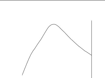
Figure 23. Energy comparison for solvated met-enkephalin. Minimum and maximum potential energies versus bin number are plotted for three temperatures: T ¼ 0 K, 250 K, 500 K.

A specific heat profile was also derived for solvated met-enkephalin in order to understand how the dominance of these extended cluster geometries affect the folding transition. These results are shown in Fig. 24. As with isolated metenkephalin, a folding transition is indicated by the peak in the specific heat, which, in this example, occurs between 275 and 300 K. This represents a significant change in average energy, which accompanies the collapse from an ensemble of extended conformations (EE*E and E*EE clusters) to the more compact ground-state cluster. For the solvated met-enkephalin example, this transition is clearly illustrated by the cluster analysis and the structure plots given in Fig. 21.

B.Structure Refinement with Sparse Restraints

To effectively determine protein function, it is important to predict the threedimensional structure of the macromolecule. Over the last several decades a number of experimental and theoretical approaches have been developed and refined in order to achieve this goal. Experimentally, there now exist two basic techniques used to perform protein structure refinement. The first, X-ray crystallography, relies on the ability to crystallize the protein so that diffraction patterns can be used for sufficient resolution. These requirements have limited

the applicability of this technique. A more powerful method, NMR (nuclear magnetic resonance) spectroscopy, is based on solution measurements of the system. Several key developments, including multidimensional NMR experiments, have resulted in the ability to determine solution structures for proteins consisting of over 200 residues.

This section focuses on the development of a novel approach for protein structure prediction via experimental NMR restraints. Traditionally, the protein folding global optimization problem involves a progression of unconstrained minimizations. However, the introduction of experimentally derived or artificial restraints can be used to recast the fundamental protein folding problem as a constrained global optimization problem. The constraints, through reduction of the feasible search space, serve two important purposes: (1) to attempt to correct any deficiencies of the energy model and (2) to focus the efforts of the global optimization algorithm.

This constrained approach is applied to the NMR structure prediction problem, although a variety of restraint information could be used. The proposed constrained formulation differs from traditional NMR approaches in several fundamental ways. First, the energy model is represented by a detailed full atom force field, rather than simplified nonbonded potential terms. This should make the approach especially effective when the number of NMR restraints per residue decreases; that is, the accuracy of the energy model becomes more significant. In addition, traditional solution approaches apply target function distance geometry or simulated annealing to unconstrained problem formulations in which restraints are represented by penalty function approximations. The solution of the constrained formulation requires the use of constrained local optimization solvers and an overall global optimization framework for nonlinearly constrained problems. This is accomplished through the application of the ideas of the aBB deterministic global optimization approach [15–18,73]. aBB-based global optimization techniques have also been applied to NMR-type structure prediction problems [92,93].

Because the location of the global minimum relies on effectively solving constrained local optimization problems, convergence to the global minimum can be enhanced by consistently identifying low-energy solutions. These observations illustrate the need for reliably locating low-energy feasible points for initializing the constrained local optimization routine. Along these lines, a combined torsion angle dynamics (TAD) and simulated annealing scheme has been implemented within the context of the global optimization framework. TAD has recently been shown to be more effective than Cartesian coordinate dynamics [94,95]. In this case, the degrees of freedom are rotations around single bonds, which reduces the number of variables by approximately tenfold because bond lengths, bond angles, chirality, and planarities are kept fixed at optimal values during the calculation.

deterministic global optimization and ab initio approaches 339

1.Energy Modeling

Basic data obtained from NMR studies consist of distance and torsion angle restraints. Once resonances have been assigned, nuclear Overhauser effect (NOE) contacts are selected and their intensities are used to calculate interproton distances. Information on torsion angles are based on the measurement of coupling constants and analysis of proton chemical shifts. Together, this information is used to formulate a nonlinear optimization problem, the solution of which should provide the correct protein structure. Typically, a hybrid energy function of the following form is employed:

The energy, E, specified by this target function includes a chemical description of the protein conformation through the use of a force field, Eforcefield. The force field potentials are generally much simpler representations of all atom force fields. The distance and dihedral angle restraints appear as weighted penalty, ENMR, terms that should be driven to zero.

The second term of Eq. (57) can be rewritten as

Here Edistance and Edihedral represent the violation energies based on the distance and dihedral angle restraints, respectively. These functions can take several forms, although a simple square well potential is commonly used. The expressions also include a summation over both upper and lower distance violations; for

example, Edistance ¼ Edistanceupper þ Edistancelower . When considering upper distance restraints, this becomes

The squared violation energy is considered only when the calculated distance dj exceeds the upper reference distance djupper. This squared violation can then be

multiplied by a weighting factor Aj. A similar contribution is calculated for those distances that violate a lower reference distance, djlower:

For dihedral angle restraints the functional form is similar to that of Eqs. (59) and (60). As before, the total violation, Edihedral, is a sum over upper and lower

and lower (olowerj ) bounds on the variable values. However, due to the periodic nature of these variables, a scaling parameter must be incorporated to capture the symmetry of the system. Furthermore, by centering the full periodic region

on the region defined by the allowable bounds, all transformed values will lie in the domain defined by [olowerj HWoj ; oupperj þ HWoj ], where HWoj is

The force field energy term, Eforcefield of Eq. (57), models the nonbonded interactions of the protein, which can consist of simple or more detailed energy functions. In practice, when considering NMR restraints, force field terms are often simplified to include only geometric energy terms such as quartic van der Waals repulsions. Such functions neglect rigorous modeling of energetic terms in order to ensure that experimental distance violations are minimized. In fact, a basic representation for this target function would be

Here the Edistance function includes additional distance restraints to avoid van der Waals contacts. Notice that when all restraints are satisfied, the objective function is driven to zero.

A detailed modeling approach is proposed by using the ECEPP/3 force field [38]. When considering an unconstrained minimization, this approach provides the following objective function:

In contrast to Eq. (63), the detailed energy modeling greatly increases the complexity of the objective function. It should also be noted that the transformation from Cartesian to internal coordinate space results in highly nonlinear

deterministic global optimization and ab initio approaches 341

functions. That is, there is not a one-to-one correspondence between distances and internal coordinates. The advantage for working in dihedral angle space is that the variable set decreases, with the disadvantage being the increased nonconvexity of the energy hypersurface.

2.Global Optimization

The determination of a three-dimensional protein structure defines an optimization problem in which the objective function may correspond to one of the target functions outlined in the previous section. For the simple case, the formulation becomes

A standard procedure for addressing this global optimization problem consists of a combination of simulated annealing and molecular or torsional angle dynamics [96]. Generally, multiple initial conformers are generated and optimized to provide a set of acceptable structures. Typically, a set containing on the order of 100 acceptable conformers may be identified, from which a subset of similar structures (approximately 20) are used to characterize the system. The simulated annealing protocol is incorporated in an attempt to reduce trapping in local minimum energy wells.

However, the minimization of complex target functions necessitates the use of rigorous global optimization techniques. For the detailed target function, given by Eq. (64), the unconstrained formulation is similar to formulation (65). Through the use of the constrained optimization approach, the dihedral angle bounds are implicitly included as box constraints. Furthermore, distance restraints are treated explicitly. This reformulation removes both Edihedral and Edistance from the target function, leaving only Eforcefield:

Here i ¼ 1; . . . ; Nf corresponds to the set of dihedral angles, fi, with fLi and fUi representing lower and upper bounds on these dihedral angles. In general, the lower and upper bounds for these variables are set to p and p, although appropriate bounds derived from NMR data are also suitable.

3.Torsion Angle Dynamics

Standard unconstrained molecular dynamics simulations have been used extensively to model the folding and unfolding of protein systems [97–99]. In

addition, several methods for NMR structure calculation have been based on molecular dynamics in Cartesian space [96]. Torsion angle dynamics differs from traditional molecular dynamics in that bond lengths and bond angles are fixed at equilibrium values, thereby allowing for a transformation from the Cartesian to the internal coordinate system. The constraints on the systems also dampen high-frequency motions, which permits the use of longer time steps during the numerical integration of the equations of motion. The use of TAD in place of conventional MD has been found to improve the efficiency of NMR structure prediction [94,95].

A major disadvantage for employing TAD in place of Cartesian MD is that the equations of motion become much more complex for the constrained system. For unconstrained Cartesian MD the accelerations of the atoms can be calculated independently due to the decoupled nature of the equations of motion. The addition of constraints to the Cartesian system transforms the equations from a system of ODEs to a system of differential algebraic equations (DAEs). The alternative to solving this system of DAEs is to transform the equations of motion to the internal coordinate reference frame. In this case, the solution of a linear matrix equation in each time step is required, which, due to the highly coupled structure of the equations, scales as a cubic function of the number of degrees of freedom (torsion angles). To avoid the potentially prohibitive computational cost required for the solution of the equations of motion, a fast recursive algorithm, which scales linearly with the number of torsion angles, was implemented. The algorithm is based on spatial operator algebra that has been used to simulate the dynamics of astronautical and robotic equipment [100].

The algorithm solves for the torsional accelerations, : y

The ability to calculate the accelerations recursively relies on the chainlike structure of the protein, in which each node of the chain represents a rigid body. These rigid bodies consist of one atom or a cluster of atoms whose relative positions are fixed. To simplify the explanation of the algorithm, an unbranched chain will be considered, although the approach can be easily extended to branched systems. For this simple case, the first rigid body, at one end of the chain, defines the base (k ¼ 0), while the last rigid body, at the other end of the chain, defines the tip (k ¼ N). The rotatable torsion angle between bodies k and k 1 is defined as yk.

deterministic global optimization and ab initio approaches 343

The framework of the algorithm to calculate can be broken down into three y

steps:

Step 1. A recursion from the base to the tip is required to calculate the positions, spatial velocities, Coriolis and gyroscopic terms for each of the rigid bodies. To proceed, the 6 6 spatial transformation matrix, fk, between rigid bodies k and k 1 must first be defined:

Here I3 and O3 denote the 3 3-dimensional identity and zero matrices,

~

while the l operator refers to the cross-product tensor associated with rk rk 1, where rk is the position vector that defines the reference frame for rigid body k. The spatial velocity, Vk, can be computed from the following relation:

The spatial velocity is a six-dimensional vector that combines both the

three-dimensional angular, o, and linear, v, velocities:

Vk ok vk

Hk is also a six-dimensional vector with the first three elements corresponding to the unit vector, ek, in the direction of the bond forming

the connection between rigid bodies k and k 1:

The Coriolis and gyroscopic terms, ak and bk, respectively, can then be calculated using the following relationships:

Both ak and bk are six-dimensional vectors. mk, Yk, and Jk represent the mass, the center-of-mass vector, and the 3 3 inertia matrix for the rigid body, respectively. Finally, the spatial inertia, Lk, of the rigid body about the reference frame is given by the following 6 6 matrix:

Step 2. The next step requires a backward recursion from the tip, k ¼ N, to the base, k ¼ 1. The recursion is used to store a number of auxiliary quantities needed for the final forward recursion to calculate the accelerations. In addition, the gyroscopic terms, bk, and the spatial inertia terms, Lk, calculated in step 1 can be used to initialize two auxiliary quantities, zk and Pk, respectively. Both Pk and zk are updated recursively using the following intermediate terms:

Here Dk and Ek denote scalar quantities, whereas Gk is a six-dimensional vector. The final equation requires the gradient of the potential function, rEk. The recurrence relationships for Pk 1 and zk 1 are given by:

Step 3. A final forward recursion from the base to the tip is used to obtain the

values. The six-dimensional vector k is used to store intermediate y a

quantities, with ak equal to a vector of zeroes for k ¼ 0.

The following recursion relation is used to update the values of ak:

For branched molecular structures, each node can potentially spawn more than one child so that both the inward and outward recursions must be modified. In the case of an inward recursion, the results from each of the child nodes must be summed up before moving up one level. In the case of the outward recursion, each of the node branches requires a separate recursion.

The TAD is carried out using simulated annealing, with temperature control provided by coupling to an external bath [101]. This coupling provides a means for forcing or damping the torsional velocities using the following scaling factor at time t:

s

fT ¼ 1 1 þ T0 ð83Þ b bTðtÞ

deterministic global optimization and ab initio approaches 345

In this equation, b is a force constant, while T0 is the bath temperature and TðtÞ is the actual temperature. The actual temperature is calculated from the kinetic energy, Ekinetic, with the following relationship:

where kB is the Boltzmann constant. The value for fT is used to scale the torsional velocities:

Once torsional velocities have been determined, the accelerations, , can be y

calculated using the recursive algorithm outlined above. A basic leap-frog technique is then employed to calculate velocities at the half-time step, which can be used to calculate torsional positions, y, and new estimated velocities at the full-time step.

4.Algorithmic Steps

The algorithmic steps for the constrained aBB approach can be generalized to any force field model or routine for solving constrained optimization problems. Here, the aBB approach is interfaced with PACK [74] and NPSOL [28]. PACK is used to transform to and from Cartesian and internal coordinate systems, as well as to obtain function and gradient contributions for the ECEPP/3 force field and the distance constraint equations. NPSOL is a local nonlinear optimization solver that is used to locally solve the constrained upper and lower bounding problems in each subdomain.

The implementation can be broken down into two main phases: initialization and computation. The basic steps of the initialization phase are as follows:

1.Choose the set of global variables. Because the bounds on these variables will be refined during the course of global optimization, they should be selected based on their overall effect on the structure of the molecule. In this work (and in general) the f and c dihedral angles provide the largest structural variability and are chosen to constitute the global variable set.

2.Set upper and lower bounds on all dihedral angles (variables). If information is not available for a given dihedral angle, the variable bounds are set to [ p, p]. Because a constrained local optimization solver is used, these box constraints are strictly enforced.

3.Identify the set of NOE-derived distance restraints to be used in the constraints. In general, this set can include all intraand inter-residue restraints. In this work, only backbone sequential and medium to