Friesner R.A. (ed.) - Advances in chemical physics, computational methods for protein folding (2002)(en)

dα1,α4

d2

d1

Figure 45. Alpha-helical ground state of unsolvated tetra-alanine, with the hydrogen bonds indicated.

The distance between a-carbons is only a crude measure of hydrogen bonding. A more direct measure is the distance between the nitrogen-bonded hydrogen atom and the oxygen atom that shares it. It turns out there are two candidate hydrogen bonding distances, as indicated in Fig. 45. These distances

only the ground state satisfies both inequalities. Apparently there are two hydrogen bonds which stabilize the a-helix in tetra-alanine.

We tabulated the average value and standard deviation of the reaction coordinate indicators for da1;a4 , d1, d2, and d1 þ d2 in Table XXXIII. The

motivation of including d þ d among the distance parameters is similar to that

P 1 2

of including i ci. Because there are two hydrogen bonds to form, it makes

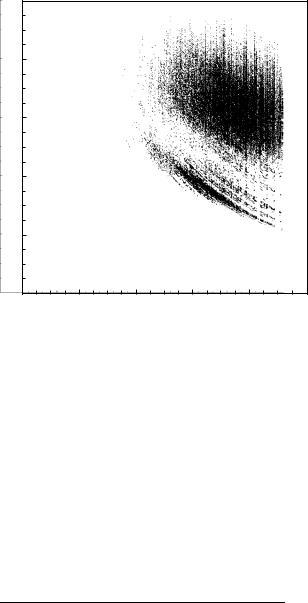
D =S ¼ 0:587. A scatter plot of D =S vs. d=D for d1 þ d2 is given in Fig. 46.

7.Solvated Tetra-Alanine

We next studied tetra-alanine in solvation. We used the ECEPP/3 potential energy surface coupled with the volume method for calculating solvation energies using the Reduced Radius Independent Gaussian Sphere (RRIGS) approximation.

deterministic global optimization and ab initio approaches 387

1

0.8

0.6

D 2/S

0.4

0.2

d /D

Figure 46. Scatter plot of reaction coordinate indicators for d1 þ d2 for each pathway. Only pathways of length 11 or less with all transition rates exceeding 1010 Hz are used (92,216 pathways).

We determined the minima and first-order saddles by applying a brute force eigenmode-following search (Eigenmode III) with a 68 grid of start points, just as we did for unsolvated tetra-alanine. The results of this search can be found in Table XXXIV.

Of the 66,228 minima, we found one a-helical conformation, min.1 (aaaa), and one extended conformation, min.874 (bbbb). The potential energy (which includes the solvation energy) and free energy (which includes contributions from the vibrational entropy) of these two states can be found in Table XXXV.

TABLE XXXIV

Eigenmode III Results for Solvated Tetra-alanine

The first thing to notice is that, although the a-helical conformation has the lowest potential energy (and hence the lowest free energy at T ¼ 0 K), the

reduces the energy gap from 11:6 kcal/mol to 4:4 kcal/mol. The entropic term in the free energy is more than enough to overpower this energy gap and reduce the free energy of the extended conformation below that of the a-helical ground state. This has significant implications.

We calculated the free energies of all the minima in order to determine the equilibrium probability distribution (see Section IV.C.2). We found that the several hundred lowest free energy minima have about the same free energy, and that no single minimum has an equilibrium occupation probability which exceeds 0:004. This is in stark contrast with unsolvated tetra-alanine, where the ground state had an equilibrium occupation probability of 0:748, and the lowest three potential energy states accounted for 0:936 of the total equilibrium probability.

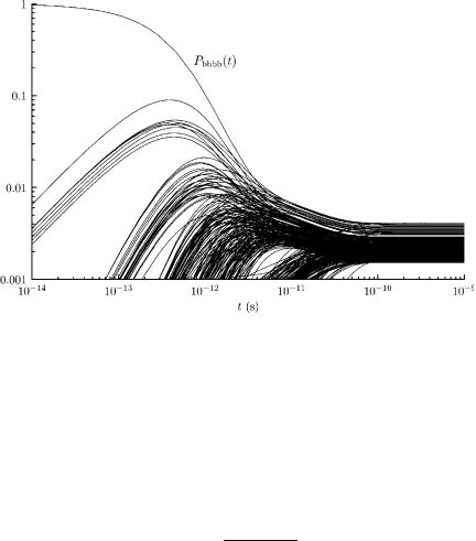
As a check, we calculated the transition rate matrix for solvated tetra-alanine at T ¼ 300 K, and we also solved the Master equation starting with the extended conformation at t ¼ 0 sec. We plotted the time evolution of the occupation probabilities of the 300 lowest free energy states. That plot is given in Fig. 47. The equilibrium probability distribution is achieved in about 10 10 sec.

It seems likely that solvated tetra-alanine exhibits liquid-like behavior at T ¼ 300 K. To be sure, we need to verify that the several hundred minima that share the equilibrium probability distribution do not occupy the same region of configuration space. If that were the case, the potential energy surface would have one deep basin with a rough bottom. The true characteristics of a liquid-like molecule is that it randomly (and quickly) samples widely distinct configurations. By plotting the distribution of minima on four ðf; cÞ plots (not shown), we reached the conclusion that the minima that share the equilibrium probability distribution do occupy distinct regions of configuration space.

If solvated tetra-alanine is to be liquid-like at T ¼ 300 K, then there must be a phase transition. This should show up as a peak in the heat capacity versus temperature plot. The heat capacity can be calculated by calculating energy

deterministic global optimization and ab initio approaches 389

Figure 47. Time evolution of the extended conformation and the 300 lowest free energy states of solvated tetra-alanine at T ¼ 300 K. No single state has an equilibrium probability that exceeds 0.004.

fluctuations at equilibrium

where equilibrium averages may be calculated from free energies

P

q e Fi=kT hqieq ¼ Pi i ei Fi=kT

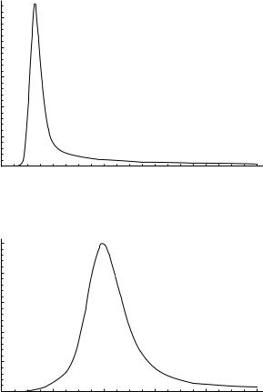
We calculated Cv as a function of T for temperatures ranging from (just above) 0 K to 1000 K for both solvated and unsolvated tetra-alanine. The plots are given in Figs. 48 and 49. The transition temperatures are given by

Tsolsolv liq ¼ 130 K Tsolunsolvliq ¼ 395 K

The lower transition temperature for solvated tetra-alanine can be traced back to the reduction in the energy gap between the a-helical ground-state conformation and the other higher-energy states, including the extended conformation, and

deterministic global optimization and ab initio approaches 391

Figure 50. Overall framework for the dynamical study of a given peptide sequence.

The stationary point search generally proceeds as follows. First, an initial sample of minima and or transition states is generated using one of the global optimization methods (aBB, CSA, or grid search). Additional stationary points can be generated, if needed, by performing uphill searches from minima to saddle points, or downhill searches from saddle points to minima, or by interpolating widely separated minima to locate new minima in between

(‘‘fill’’). Similar minima and transition states may be combined by clustering, if desired.

Once an adequate sample of minima and transition states has been found, we begin the dynamical analysis. Connectivity between minima and transition states has already been determined by the triples calculation (i.e., downhill searches). The free energy of each stationary point is calculated (using the vibrational frequencies), and from that the transition rates may be calculated. Then we can construct a Cv vs. T plot, determine equilibrium probability distributions, solve the Master equation, construct the rate disconnectivity graph, and perform a full pathway analysis.

1.Local Stationary Point Search Methods

Eigenmode-Following Search. Eigenmode-following search algorithms are essentially sophisticated variations of the Newton–Raphson method applied to the equations qV=qxi ¼ 0. We employ the version introduced by Tsai and Jordan [145]. At each iteration, the Hessian may be updated by direct calculation, or by BFGS (minimum search only) or Powell updating (with occasional direct calculation) [159–161]. We generally used the Powell updating for the uphill searches and a full Hessian calculation for the downhill searches, so as to ensure that the correct connectivity is determined.

The Newton–Raphson step is given by

x ¼ H 1g ¼ X gi ei

i bi

where g and H are the gradient and Hessian, respectively, bi and ei are eigenvalues and eigenvectors of H, respectively, and gi is the component of the gradient in the direction of ei. The Newton–Raphson algorithm tends to locate stationary points that have the same signature (i.e., number of negative eigenvalues) as the Hessian matrix at the starting point. More specifically, potential energy tends to be minimized along modes for which bi > 0, and it tends to be maximized along modes for which bi < 0. Eigenmode-following algorithms circumvent this limitation by ‘‘shifting’’ some of the eigenvalues to change their sign, so that the ‘‘eigenvalues’’ used to construct the step have the desired signature. Thus, if a minimum is sought, then all eigenvalues are rendered positive by shifting the negative bi’s to positive values. If a first-order saddle is desired, then eigenvalues are shifted as needed so that one specific eigenvalue is negative. If the Hessian already has the required signature, no shifting takes place—the search essentially becomes a Newton–Raphson search in the vicinity of the saddle point. Eigenmode-following searches, when they converge, virtually always converge to a saddle point of the correct saddle order.

deterministic global optimization and ab initio approaches 393

When searching for a first-order saddle from a starting point in the vicinity of a minimum, there is some question as to which eigenvalue should be shifted to a negative value (i.e., which eigenmode to follow ‘‘uphill’’). There are two possible answers:

1.At each iteration, follow the mode with the smallest eigenvalue.

2.Choose a specific mode at the starting point, and continue to follow that ‘‘same’’ mode as each step is taken. Eigenmodes at each subsequent step are identified with eigenmodes at previous steps by maximum overlap.

In the first case, it is automatically the case that at any point where the Hessian has the correct signature, no eigenvalue shifting takes place at all, and the Newton–Raphson step is taken. In the second case, a specific mode is selected, which often does not start out as the lowest eigenvalue mode. However, as the selected mode is driven uphill, its eigenvalue decreases, eventually causing that mode to overtake the other modes in becoming the lowest eigenvalue mode. Eventually the eigenvalue is driven to a negative value, after which the first-order saddle will be found.

SUMSL. The SUMSL algorithm [162], which is made available as part of ECEPP/3 [38], is designed to find local minima in the vicinity of a starting point. It employs the BFGS updating method for the Hessian. It is specifically designed for minimum searches and, as such, is generally much more efficient than the eigenmode-following algorithm.

2. Methods for Finding Minima and First-Order and Higher-Order Transition States

aBB Stationary points of all orders are generated by solving the stationary conditions

qV

qxi ¼ 0 i ¼ 1; . . . ; Nx

using the aBB method described in Sections II.B and IV.B. This algorithm offers a theoretical guarantee of enclosing all solutions within the starting region in a finite amount of time.

CSA. The Conformational Space Annealing (CSA) algorithm attempts to reach the global minimum (free) energy conformation by a combination of genetic, annealing, and buildup algorithms [115,153,154]. The user provides an initial bank of minima (usually by locally minimizing randomly selected points). Seed points are selected from the bank and modified according to prespecified rules. The modified points are then minimized by local search, and then considered for

introduction into the bank, possibly replacing a point which is already there. If the candidate point falls within a certain ‘‘cutoff distance’’ from any other point in the bank, the candidate point and the bank point closest to it are compared. Otherwise, the candidate point is considered to be in its own ‘‘class,’’ and it is compared with all other points in the bank. In either case, the highest (free) energy point is discarded. The ‘‘cutoff distance’’ is initialized to one-half the average distance between points in the initial bank, and it is annealed down by a fixed factor every iteration.

Termination conditions include one or more of the following:

1.Iteration count limit.

2.Round limit. Each round ends after every point in the current bank has been used as a seed point.

3.(Free) energy lower limit.

4.Update counter limit. The ‘‘update counter’’ is incremented whenever the fraction of candidate points which actually make it into the bank is sufficiently small for a given number of minimizations.

5.Stop file. The user can stop the algorithm by creating a special file whose existence is checked each iteration.

Virtually all of the effort is spent performing the local minimizations of the modified seed points. The parallel version of this algorithm divides the modified seed points among all of the processes (including the master process) to be minimized in parallel. The master process handles the rest of the algorithm.

Grid Search. A sampling of stationary points of a specified order (first-order saddle or minima, generally) is found by initiating an eigenmode-following search from each point on a specified grid to a saddle point of the specified order. After the searches are completed, duplicate points are thrown out. This algorithm requires one search for each grid point, and thus the time requirements depend exponentially on the number of variables for which alternative values are provided for the grid. It is therefore unsuited for large problems, but yields good results for small problems (e.g., tetra-alanine, discussed in Section IV.C).

The parallel version of this algorithm divides the gridpoints among all of the processes (including the master process), which then perform the searches. The results are sent back to the master process.

Uphill Search. First-order saddle points are found by performing eigenmodefollowing searches ‘‘uphill’’ from each minimum. For every minimum and every choice of eigenmode, an initial step is taken along that mode (in each of the two possible directions), followed by an eigenmode-following search along that mode to a first-order saddle. A total of 2N searches are required for each minimum, where N is the number of eigenmodes. One may alternatively restrict

deterministic global optimization and ab initio approaches 395

the number of modes followed for each minimum. The resulting saddles are collected and duplicates are removed.

The parallel version of this algorithm divides the minima among all of the processes (including the master process), which then perform all of the required searches. The results are sent back to the master process.

Triples Calculation. The connection between first-order saddles and the minima they connect are found by performing a minimization on each side of the saddle point. An initial step from the saddle point is taken in each of the two directions along the eigenmode corresponding to the negative eigenvalue, each followed by a minimization. Minima found this way are compared with minima that have been found previously, and duplicates are discarded in favor of the previously found minima. This algorithm may also be used to locate previously unknown minima by downhill search from a saddle point, in which case the new minima are retained.

The parallel version of this algorithm divides the saddle points among all of the processes, which then perform the necessary minimizations. As the saddles and minima are sent back to the master process, duplicate minima are discarded in favor of previously determined minima.

Fill. ‘‘Fill’’ refers to the act of filling in a ‘‘scaffolding’’ of minima (such as might be obtained by a CSA run) by searching for additional minima between pairs of minima found in the initial set. The reason why this may be necessary is because the minima generated by the CSA algorithm are often too far apart for connections between them to develop after a single uphill/downhill search (this is practically by design of the CSA algorithm, which spreads itself thin so as to sample a large portion of the conformational space).

A ‘‘distance cutoff’’ and a ‘‘coordination number’’ are provided, along with an initial set of minima. Ideally, this algorithm will first cluster the points according to the distance cutoff (i.e., split the points into equivalence classes, where two points are equivalent if they can be connected to one another by a ‘‘path’’ involving points which are within the cutoff distance from each other). Then each cluster will be paired with the N clusters closest to it in distance, where N is the coordination number. For every pair of clusters generated this way, additional points will be added along the line joining the two clusters (more specifically, along the line joining the two representative points in the two clusters which are the least distance apart). The points will be uniformly spaced, and the number of points chosen is the least number which results in each point being within the cutoff distance from its nearest neighbor. The new points can then be used as starting points for minimization.

For practical reasons, the algorithm actually proceeds as follows. Every point is considered in turn. Distances from that point to every other point are first