Friesner R.A. (ed.) - Advances in chemical physics, computational methods for protein folding (2002)(en)

and the measure of convexity. In order to develop a meaningful comparison of relative free energies, the total partition function [i.e., the denominator of Eq. (47)] must include an adequate ensemble of low-energy local minima, as well as the global minimum energy conformation.

These probabilities can be used to estimate the occupancy of each individual basin, or summed in order to calculate cumulative probabilities for an ensemble of structures exhibiting similar physical or energetic properties. It should be noted that the determination of free energy using the harmonic approximation does not require the explicit inclusion of a contribution based on the density of states. That is, the harmonic approximation decomposes the energetic states within a basin of attraction into one energetic value represented by the local minimizer of the basin. In contrast to counting methods, which estimate probabilities based on the density of states, the contribution of each structure should be accounted for only once. Therefore, using the harmonic approximation requires a structural comparison of all local minimizers.

The probabilities obtained through the harmonic approximation can also be used to calculate thermodynamic quantities. Once the set of unique minimizers has been identified, these structures can be ranked according to their free energy values and then divided into bins of a specified energy width. Probabilities for each bin can be calculated by summing the individual probabilities [as defined in Eq. (47)]:

g¼1

Here Papproxj signifies the probability for energy bin j. The summation includes the nj individual probabilities (papproxg ) belonging to bin j. Average thermodynamic quantities can now be estimated using equations with the following

j

Here the total average energy, hEiT , is calculated by summing the bin probabilities multiplied by the mean energy of bin j, hEij.

7.Free Energy Problem Formulation

As before, the energy minimization problem for proteins is formulated as a nonconvex nonlinear optimization problem. The inclusion of free energy modeling into the protein folding problem does not change the general formulation. However, an additional condition must be satisfied; that is, an ensemble of local minimum low-energy conformations must be generated along with the global minimum energy conformation. Once this ensemble has been compiled, a free

deterministic global optimization and ab initio approaches 317

energy ranking can be performed using the harmonic approximation presented in the previous section.

Several rigorous methods can be envisioned for locating local minimum energy conformations using the aBB deterministic global optimization approach. As an introduction to the ideas used here, two rigorous approaches for finding all local minimum energy conformations are discussed.

The first method relies on the introduction of a single inequality constraint to the problem formulation given by (34). The new formulation is:

The additional constraint requires that the objective function values be larger than the energy value at some local (or global) minimum, as denoted by E , plus a positive parameter, E . When E ¼ 0, the solution of the corresponding global optimization problem will give the best local minimum energy conformation with an energy larger than E . The original formulation given by (34) is actually a special case of this problem in which E ¼ 1 and E ¼ 0. That is, in (34) no bounds are placed on the value of the objective function, E. The global minimum energy conformation is only required to take some finite value. In order to locate all local minima, a set of global optimization problems must be solved iteratively with updating of the parameter E .

The problem of finding all local minimum energy conformations can also be formulated as a single global optimization problem, which can be deterministically solved using the aBB algorithm [23]. This method stems from the idea that all stationary points (i.e., minima, maxima, and transition states) of the energy hypersurface satisfy the constraint rEðyÞ ¼ 0. This can be written as:

Here Ny represents the total number of dihedral angles defined by the variable set y. The problem of finding local minima is equivalent to finding all solutions of Eq. (51) for which the Hessian of E is positive definite.

The problem posed in Eq. (51) involves the solution of a system of nonlinear equations. The identification of all multiple global solutions requires the use of a deterministic global optimization method, as outlined in Section II.B. The application of this method to protein systems will be described fully in Section IV.B.

Both methods for rigorously locating all local minimum energy conformations have some disadvantages. On one hand, the first approach should effectively locate low energy conformers in order of increasing energy. However, locating each minimum requires the solution of a full global optimization problem. The second approach avoids this drawback because it can be solved as a single global optimization problem. However, when dealing with a high-dimensional search space, the number of necessary subdivisions may be computationally inhibitive. In addition, this method will potentially locate stationary points other than local minima. Therefore, the development of other methods for locating low-energy local minimum energy conformations were pursued.

8.Ensemble of Local Minimum Energy Conformations

Because the number of local minima on a given energy hypersurface may become astronomically large (e.g., the number of local minima for met-enkephalin is estimated to be on the order of 1011 [77]), methods that do not necessarily provide all local minima were developed. Specifically, it was determined that the generation of ensembles of low-energy conformers is possible through algorithmic modifications of the general aBB procedure. Rigorous implementation of the global optimization algorithm requires the minimization of a convex lower bounding function in each domain. The unique solution y for each lower bounding minimum can then used as a starting point for the minimization (or function evaluation) of the original energy function in the current domain. In the case of local minimization, each partitioned region provides a single minimum energy conformation as the algorithm proceeds. Using this information, along with the global minimum energy conformation, a list of low-energy conformers can be constructed.

A method for increasing the number of local minima produced within each subdomain would involve the selection of multiple random starting points for minimizing the upper bounding function. At first, this approach appears to be equivalent to choosing random points for local minimization. Initially, when the subdomains constitute significant portions of the original domain space, this is the case. However, as the separation between lower and upper bounds

deterministic global optimization and ab initio approaches 319

decreases, the subdomains are localized in regions of low energy. Therefore, the random point selection is localized in regions that contain low-energy local minima.

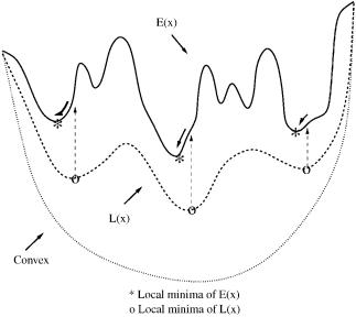
However, this approach does not take advantage of the information provided by the lower bounding functions. Rigorously, these functions possess a single minimum in each subdomain. Because the choice of a affects the convexity of the lower bounding functions, the a values can be modified to ensure a certain nonconvexity in these functions. In this case, the lower bounding functions possess multiple minima, and these functions can be minimized several times in each domain. In addition, because the lower bounding functions smooth the original energy hypersurface, the location of these multiple minima provide information on the location of low-energy minima for the upper bounding function. Therefore, by using the location of the minima of the lower bounding function as starting points for local minimization of the upper bounding function, an improved set of low-energy conformations can be identified. As before, these conformations are also localized in those domains with low-energy as the subdomains decrease in size. This Energy-Directed Approach (EDA) is represented schematically in Fig. 17.

Figure 17. Using multiple lower bound minima to find low-energy conformers of the upper bounding function.

The basic steps of the algorithm, which are qualitatively similar to those outlined in Fig. 12, are as follows:

1.The initial best upper bound is set to an arbitrarily large value. The original domain is partitioned along one of the global variables. a values are initially chosen to be constant (a ¼ a0) for all global variables.

2.The lower bounding function (L) is constructed in each hyper-rectangle. Three local minimization are performed using the following procedure:

a.Fifty random points are generated and used for function evaluations.

b.The point with the minimum value is used as a starting point for local minimization of L using NPSOL, with calls (through PACK) to ECEPP/ 3 and possibly the RRIGS solvation module.

c.The unique solutions are stored.

If the minimum valued solution (of all local minima of L in this subdomain) is greater than the current best upper bound the subdomain is fathomed.

3.The unique local minima (points) for L are used as initial starting points for local minimizations of the upper bounding function (E) in each hyperrectangle. Again, the appropriate calls are made to PACK and the potential and solvation energy modules. Two additional minimizations are performed using the following procedure:

a.Fifty random points are generated and used for function evaluations.

b.The point with the minimum value is used as a starting point for local minimization of E using NPSOL, with calls (through PACK) to ECEPP/3 and possibly the RRIGS solvation module.

In all cases, the UBC (upper bound check) module is also called. UBC checks that the absolute value of each gradient in the objective function gradient vector is below a specified tolerance (10 6 kcal/mol/deg). If a gradient does not satisfy this check, the corresponding variable bounds are incrementally increased and the problem is solved with the previous point used as the initial starting point. This process is repeated until the gradient constraints are satisfied or an iteration limit is exceeded. UBC also employs algorithms to calculate the second derivative matrix [75], which is used to verify that the upper bound solution is a local minimum; that is, the Hessian matrix must be positive semidefinite. If the matrix is not positive semidefinite or the gradient checks are not satisfied, the upper bound solution is rejected. All local minima are stored.

4.The current best upper bound is updated to be the minimum of those thus far stored.

deterministic global optimization and ab initio approaches 321

5.The hyper-rectangle with the current minimum value for L (this is the minimum value of all local minima of L in each subdomain) is selected and partitioned along one of the global variables. All a values are updated according to the following rule:

In this equation a0 refer to the initial values from Step 1. R is a reduction parameter (0 < R 1), and L refers to the current level in the branch and bound tree. For R ¼ 1 the a values are kept constant at the initial value, a0.

6.If the best upper and lower bounds are within the E tolerance, or a maximum iteration limit has been exceeded, the program will terminate, otherwise it will return to Step 2.

A second approach incorporates free energy information into the branch and bound algorithm. Specifically, harmonic entropic contributions are calculated and included at each minima of the upper and lower bounding functions. In this way, the progression of lower and upper bounds includes a temperaturedependent entropic term. A similar modification to the Monte Carlo minimization method has also been proposed [87] and has been shown to be effective in locating low-energy conformers of peptides [88,89].

The problem formulation is identical to the one given in (34). That is, the minimization of E and L are still performed using only potential and solvation energy contributions. However, once local minima have been located, the free energy is calculated by the following expression:

This equation is similar to Eq. (44), although the additive term f ðTÞ has been omitted because it is a function of temperature only. UMin represents the local minimum energy of E or L, and DetðHMinÞ is the determinant of the Hessian evaluated at this local minimum. The specification of a thermodynamic temperature (b ¼ 1=kBT) is required as an additional input parameter.

A single rigorous application of the aBB algorithm to this problem will result in the identification of the global minimum free energy at a given temperature. However, the goal is to identify an ensemble of low energy and, in this case, low free energy conformers so that a free energy ranking and comparison can be made. Therefore, the algorithmic steps for the Free Energy-Directed Approach (FEDA) are similar to those for EDA, with the additional evaluation of the free energy (G) at each local minima of E and L. The thermodynamic temperature used in Eq. (53) must be specified as an additional input parameter.

9.Free Energy Computational Studies

The EDA was first applied to the isolated form of met-enkephalin. All 24 dihedral angles were considered variable, with the 10 dihedral angles of the backbone residues acting as global variables (variables on which branching occurs). For both peptides, the EDA algorithm detailed above was applied 10 times. The input conditions correspond to initial a values of 5 and 10, with a subsequent reduction of these values based on the current level in the branch and bound tree.

Once the ensemble of local minima had been compiled, a set of distinct conformations was identified by checking for repeated and symmetric conformations. In addition, a conformation was only considered unique if at least one dihedral angle differed by at least 50 when comparing each pair of conformations. These conformations were then used to generate results and distributions according to energy and free energy values. Energy bins were used to characterize a group of distinct structures between a range of energy values (every 0.5 kcal/mol) relative to the global minimum energy structure. For example, Bin 1 contains structures that are 0.0–0.5 kcal/mol above the global minimum energy structure, Bin 2 contains structures that are 0.5–1.0 kcal/mol above the global minimum energy structure, and so on.

In the case of isolated met-enkephalin, the 10 (EDA) runs generated a total of 83,908 distinct local minima. The potential energy global minimum (PEGM) conformation for met-enkephalin possesses an energy of 11:707 kcal/mol. This conformation exhibits a type II0 b-bend along the N–C0 peptidic bond of Gly3 and Phe4. Essentially, this structure corresponds to the free energy global minimum (FEGM) conformation for a temperature of 0 K—that is, when entropic contributions are not included. When considering the harmonic free energy, the prediction of the FEGM can be calculated over a range of temperatures. Table XI provides information on the FEGM for temperatures ranging from 100 K to 500 K.

As Table XI shows, the PEGM persists as the FEGM at a temperature of 100 K. However, at the next three temperature points (i.e., 200 K, 300 K, 400 K) the FEGM exhibits a potential energy contribution 1.808 kcal/mol higher than the PEGM. The f and c values for this structure are also significantly different than those for the PEGM. In fact, the conformational code (B*AAAE) indicates that the central residues display an a helical configuration. At a temperature of 500 K, the FEGM structure changes again, while the potential energy difference between the FEGM and PEGM increases to 5.369 kcal/mol. These differences suggest that the inclusion of entropic contributions greatly affects the relative stability of individual low energy structures. In addition, as the temperature increases, the stability offered by entropic contributions offsets substantial differences in potential energy.

deterministic global optimization and ab initio approaches 323

TABLE XI

Dihedral Angle Values for PEGM and FEGM Structures of Isolated Met-enkephalin Using EDAa

aThe temperatures are provided in the first row. The last two rows indicate the harmonic free energy (kcal/mol) and the potential energy value (kcal/mol), respectively.

Table XII provides information on the distribution of distinct low free energy minima within 8.0 kcal/mol of the FEGM for a range of temperatures. For a given temperature the general trend indicates a large increase in the number of minima as the free energy increases above the FEGM. Several exceptions to this trend occur at high temperature and large bin number. In these cases, the number of minima remains constant or even decreases slightly. This is most likely due to an inadequate sampling of higher potential energy minima. For a given bin, it is also apparent that the clustering of low free energy structures increases with temperature. This increased density of the free energy bins indicates that increases in energy are offset by entropic contributions.

aEach bin represents a 0.5 kcal/mol range above the previous bin. The temperatures are given in the first row.

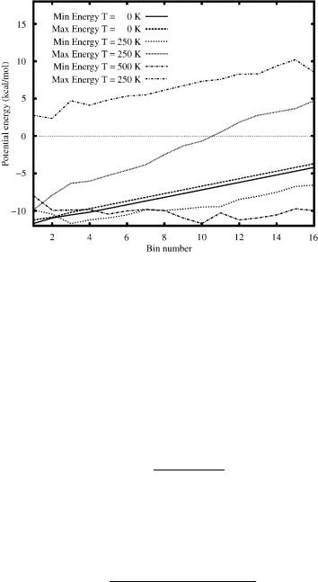
These observations are also supported by the information shown in Fig. 18. This plot displays the range of potential energy in free energy bins at temperatures of 250 and 500 K, with the potential energy bins included for comparison. As expected, the potential energy values for the free energy bins increase with increasing temperature. In addition, the range of potential energy values increases in higher free energy bins. It is interesting to note that this occurs because the minimum potential energy is relatively (i.e., within a few kcal/mol of the PEGM) low for each bin, whereas the maximum potential energy value increases in higher bins. The corresponding differences are also greater at higher temperature. For example, at 500 K some bins exhibit a 20-kcal/mol range in potential energy. These trends explain the increased number of low free energy conformers. That is, bins of low free energy contain conformers of relatively high potential energy because of their more stabilizing entropic contributions. The plot also implies that the PEGM appears in bins 3 and 10 for temperatures of 250 and 500 K, respectively.

Relative free energies were also calculated for clusters of low-energy conformers. This analysis is useful because it is difficult to capture the true accessibility of individual structures based on a pointwise approximation of entropic effects. That is, the harmonic free energy approximation does not provide a continuous free energy landscape. By clustering structures into larger

deterministic global optimization and ab initio approaches 325

Figure 18. Potential energy comparison for isolated met-enkephalin using EDA. Minimum and maximum potential energies versus bin number are plotted for three temperatures: T = 0 K, 250 K, 500 K.

groups, it is hoped that the error associated with these estimates will average out. Typically, structures are clustered by calculating and comparing root-mean- squared deviations. Because the enkephalin peptide is relatively small, structures were grouped based on the Zimmerman codes for the central residues of the peptide [90]. Specifically, for met-enkephalin, structures were said to belong to the same cluster if the central three residues possessed the same three code letters based on the Zimmerman classification [90]. The relative free energy of a cluster was calculated by the following equation:

In Eq. (54) the individual papproxi , which refers to the statistical weight based on the harmonic approximation, are summed for the set of conformations belonging to a particular cluster (C). These individual probabilities were calculated by normalizing each probability with respect to the overall probability at a given temperature: