

Friesner R.A. (ed.) - Advances in chemical physics, computational methods for protein folding (2002)(en)
.pdfab initio protein structure prediction |
235 |
Energy
3.5 |
|
|
|
|
|
|
|
|
|
|
|
|
|
|
|
|
'ARG.ARG.1' |
|
|
||
3 |
|
|
|
|
|
'ARG.ARG.2' |
|
|
||
|
|
|
|
|
|
'ARG.ARG.3' |
|
|
||
2.5 |
|
|
|
|
|
'ARG.ARG.4' |
|
|
||
|
|
|
|
|
|
'ARG.ARG.5' |
|
|
||
2 |
|
|
|
|
|
'ARG.ARG.6' |
|
|
||
|
|
|
|
|
|
|
|
|
|
|
1.5 |
|
|
|
|
|
|
|
|
|
|
1 |
|
|
|
|
|
|
|
|
|
|
0.5 |
|
|
|
|
|
|
|
|
|
|
0 |
|
|
|
|
|
|
|
|
|
|
−0.5 |
|
|
|
|
|
|
|
|
|
|
0 |
5 |
10 |
15 |
20 |
25 |
30 |
35 |
40 |
45 |
50 |
Distance
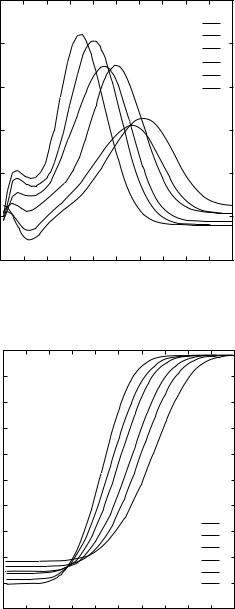
Figure 2. Size dependence of three representative terms in Eq. (4) for the amino acid pair arginine–arginine–arginine. Data for the first six size bins are shown.
Energy
2.2 |
|
|
2 |
'ARG.ILE.1' |
|
'ARG.ILE.2' |
||
|
||
1.8 |
'ARG.ILE.3' |
|
'ARG.ILE.4' |
||
|
||
1.6 |
'ARG.ILE.5' |
|
'ARG.ILE.6' |
||
|
||
1.4 |
|
|
1.2 |
|
1
0.8
0.6
0.4
0 |
5 |
10 |
15 |
20 |
25 |
30 |
35 |
40 |
45 |
50 |
|
|
|
|
Distance |
|
|
|
|
||
Figure 3. Size dependence of three representative terms in Eq. (4) for the amino acid pair arginine–isoleucine. Data for the first six size bins are shown.
236 volker a. eyrich, richard a. friesner, and daron m. standley
Energy
3 |
|
|
|
'ILE.ILE.1' |
|
2.5 |
'ILE.ILE.2' |
|
'ILE.ILE.3' |
||
|
||
|
'ILE.ILE.4' |
|
2 |
'ILE.ILE.5' |
|
'ILE.ILE.6' |
||
1.5 |
|
|
1 |
|
|
0.5 |
|
0
0 |
5 |
10 |
15 |
20 |
25 |
30 |
35 |
40 |
45 |
50 |
|
|
|
|
Distance |
|
|
|
|
||
Figure 4. Size dependence of three representative terms in Eq. (4) for the amino acid pair isoleucine–isoleucine. Data for the first six size bins.
|
7 |
|
|
|
|
|
|
|
|
|
|
|
6.5 |
|
|
|
|
|
|
|
|
|
|
|
6 |
|
|
|
|
|
|
|
|
|
|
|
5.5 |
|
|
|
|
|
|
|
|
|
|
Energy |
5 |
|
|
|
|
|
|
|
|
|
|
4.5 |
|
|
|
|
|
|
|
|
|
|
|
|
|
|
|
|
|
|
|
|
|
|
|
|
4 |
|
|
|
|
|
|
|
|
|
|
|
3.5 |
|
|
|
|
|
|
'size1' |
|
|
|
|
|
|
|
|
|
|
'size2' |
|
|
||
|
|
|
|
|
|
|
|
|
|
||
|
3 |
|
|
|
|
|
|
'size3' |
|
|
|
|
|
|
|
|
|
|
'size4' |
|
|
||
|
|
|
|
|
|
|
|
|
|
||
|
2.5 |
|
|
|
|
|
|
'size5' |
|
|
|
|
|
|
|
|
|
|
'size6' |
|
|
||
|
2 |
5 |
10 |
15 |
20 |
25 |
30 |
35 |
40 |
45 |
50 |
|
0 |
||||||||||
Distance
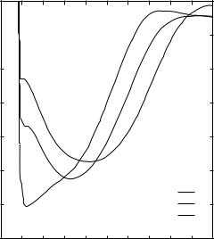
Figure 5. Density profiles for the first six size bins.
ab initio protein structure prediction |
237 |
be easily rationalized: The arginine–arginine residues are pushed apart, while the isoleucine–isoleucine interaction is attractive. The arginine–isoleucine term is repulsive is well, but the minimum values occur at shorter distances than in the corresponding arginine–arginine plots, consistent with our intuitive picture of a spheroid with hydrophilic residues residing primarily on the surface. Not surprisingly, the basic effect of the density profile is to restrict the interresidue separation as a function of protein size. Note also that the density profile is the most sensitive to protein size (although the isoleucine–isoleucine pair potential clearly decreases with size).
Figure 6 illustrates the effect of adding the excluded volume and density profile to the arginine–arginine, arginine–isoleucine, and isoleucine-isoleucine potentials, respectively, for size bin 6. We see here that the linear portions of the
˚
potential are now restricted to a small range in distance (about 6–12 A), outside of which the density profile and excluded volume become the dominant terms.
˚
The energies of each of the three residue pairs at large separation (e.g., 25 A) relative to their minimum values increase in the expected order (EIle-Ile >
EArg-Ile > EArg-Arg).
Energy
5
4.5
4
3.5
3
2.5
'ARG.ARG.6' 2 'ARG.ILE.6'
'ILE.ILE.6'
1.5
0 |
5 |
10 |
15 |
20 |
25 |
30 |
35 |
40 |
45 |
50 |
|
|
|
|
Distance |
|
|
|
|
||
Figure 6. Total energy for three representative residue pairs: arginine–arginine, arginine– isoleucine, and isoleucine–isoleucine. The data corresponds to size bin 6.
238volker a. eyrich, richard a. friesner, and daron m. standley
III. TERTIARY FOLDING SIMULATIONS: PDB DERIVED AND IDEAL SECONDARY STRUCTURES
A.Physical Model
The physical model of the polypeptide chain we use has been described previously [2]; a few minor modifications are introduced as noted below. All bond angles and bond lengths are fixed at ideal values. The variables in the optimization are the torsional angles f and c of the peptide backbone. Each residue is represented by a Ca atom and a Cb-like atom. The Cb atom position is given by the average projection of the side-chain center of mass onto the Ca–Cb bond vector.
We employ three different methods to describe the location and threedimensional structure of secondary structure elements (i.e., a-helices and b-strands). The first is to take both the sequence location and backbone angles (which are frozen during the simulation) directly from the PDB entry. This is obviously not a realistic data set in a predictive situation, but is an essential computational experiment in that it indicates what level of accuracy is possible with ‘‘perfect’’ secondary structure information. The second is the replacement of PDB backbone angles with ideal backbone angles; this separates the effects of distortion of secondary structural elements from ideal geometries from errors in location in the sequence or in length. For these two types of calculations the correct size-dependent potential is selected by evaluating the radius of the gyration of the corresponding native structure. The third is to employ predicted, rather than PDB, secondary structure (along with the use of ideal geometries for the predicted elements) and to select the correct potential by predicting the radius of gyration from the number of residues of the target [22]. We have carried out an extensive investigation in this regard, using secondary structure prediction from various secondary structure prediction servers that are available over the Internet. These results are then combined to produce genuine ab initio structural prediction. The results, while far from a robust ab initio methodology over all protein types, yield important insights into the key obstacles to ab initio prediction and are in many cases surprisingly accurate. Predictions from the CASP3 contest are also included so that comparisons can be made with the work of others. While we are not generating these predictions as a blind test, it is the case that our CASP3 calculations were carried out using our software in a completely automated fashion, with no readjustment of parameters after obtaining results for the CASP3 targets.
B.Simulation Methodology
Our simulation methodology is identical to that presented in previous publications [2], so we will describe it only briefly here. The algorithm is based
ab initio protein structure prediction |
239 |
on the Monte Carlo plus minimization (MCM) strategy proposed by Li and Scheraga [23]. This approach has proven to be extraordinarily efficacious in our previous work, and the present results reinforce our conclusions concerning its robustness and efficiency in enumerating the low-energy basins of attraction for low-resolution models such as those employed here. As in previous work [2], we have incorporated several key modifications of the algorithm, the most important of which is that the number of minimization steps is annealed as a function of the simulation temperature (i.e., more steps are taken later in the simulation), which yields a factor of 5–10 times reduction in computational effort. Finally, calculations are performed using a parallelized version of the code (an MPI implementation) on a network of PCs using Intel microprocessors and also on a large SGI Origin at the National Center for Supercomputing Applications.
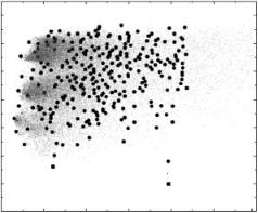
The MCM procedure produces a large number of low-energy structures. The structurally unique predictions are extracted from the raw simulation data by a clustering algorithm. Figure 7 illustrates this process for the protein 1ACP. The raw simulation data (red dots) are combined into structurally similar clusters using a procedure discussed in Ref. 24. The criterion for separating structures into clusters is that the average RMSD between clusters (calculated over all
˚
structures in a particular cluster) be at least 5 A. Clusters are represented by their lowest energy structure (black circles), which means that energies and RMSDs reported for clusters are based on their lowest-energy structure. The
1ACP
RMSD from the native structure
14 |
|
|
|
|
|
|
12 |
|
|
|
|
|
|
10 |
|
|
|
|
|
|
8 |
|
|
|
|
|
|
6 |
|
|
|
|
|
|
4 |
|
|
|
Clusters |
|
|
2 |
|
|
|
Raw Data |
|
|
|
|
|
Minimized native |
|||
0 |
|
|
|
|
|
|
5400 |
5450 |
5500 |
5550 |
5600 |
5650 |
5700 |
Energy
Figure 7. (See also color insert.) Comparison of raw data and clustered results (red dots: raw simulation data, black circles: cluster representatives, green square: locally minimized native structure).

240 volker a. eyrich, richard a. friesner, and daron m. standley
TABLE III
RMSD with Respect to the Native of the ten Lowest Energy Clusters (Represented by Their Lowest Energy Member) for the Protein 1acpa
Cluster # |
RMSD |
Energy |
N |
|
|
|
|
1 |
6.65 |
5415.43 |
43 |
2 |
5.72 |
5417.83 |
58 |
3 |
8.64 |
5420.17 |
23 |
4 |
7.54 |
5420.80 |
25 |
5 |
11.08 |
5422.82 |
31 |
6 |
9.65 |
5424.04 |
34 |
7 |
4.79 |
5427.21 |
22 |
8 |
5.91 |
5431.10 |
16 |
9 |
8.27 |
5431.23 |
12 |
10 |
12.10 |
5432.68 |
19 |
aN gives the number of structures combined into a cluster.
˚
RMSD between resulting representative structures is usually at least 5 A, but this is not guaranteed by the clustering algorithm because we use the average RMSD as the clustering criterion. For the 10 representative structures lowest in energy we list energy, RMSD with respect to the native and number of structures combined into a cluster in Table III, and the RMSD between the representative structures themselves in Table IV. Derivation of the ranks of structures (discussed below) is straightforward given the data in Table III.
The lowest-energy structure obtained from the simulations is generally highly refined, meaning that its energy cannot be lowered significantly by performing more extensive searches. Refinement of higher-energy structures, structures that do not rank first, is possible though and in some of the cases,
TABLE IV
RMSD Between the Representative Structures from the Ten Lowest-Energy Clusters for the Protein 1acp
Cluster # |
1 |
2 |
3 |
4 |
5 |
6 |
7 |
8 |
9 |
10 |
|
|
|
|
|
|
|
|
|
|
|
1 |
0.00 |
2.23 |
8.73 |
2.31 |
9.91 |
5.01 |
7.18 |
9.35 |
8.20 |
12.23 |
2 |
|
0.00 |
8.70 |
3.41 |
9.94 |
6.04 |
6.08 |
8.35 |
8.16 |
11.93 |
3 |
|
|
0.00 |
8.85 |
11.86 |
8.63 |
8.46 |
8.24 |
3.04 |
8.63 |
4 |
|
|
|
0.00 |
9.70 |
4.08 |
7.97 |
9.91 |
8.53 |
12.14 |
5 |
|
|
|
|
0.00 |
8.69 |
11.31 |
11.02 |
11.77 |
8.40 |
6 |
|
|
|
|
|
0.00 |
10.54 |
11.91 |
8.45 |
11.75 |
7 |
|
|
|
|
|
|
0.00 |
3.01 |
8.27 |
10.81 |
8 |
|
|
|
|
|
|
|
0.00 |
8.46 |
9.91 |
9 |
|
|
|
|
|
|
|
|
0.00 |
9.04 |
10 |
|
|
|
|
|
|
|
|
|
0.00 |
|
|
|
|
|
|
|
|
|
|
|
ab initio protein structure prediction |
241 |
especially the larger proteins, actually results in improved ranks. We have not yet developed the optimal refinement strategy though and therefore do not report results for this approach.
C.Comparison of the Size-Dependent Potential with Previous Results
Using PDB-Derived Secondary Structure
As a test set, we employed the subset of the 95 proteins used in Ref. 2 which are less than 100 residues and are not all b-strand. There is some overlap with the training set; but in tertiary folding, this is less of a concern than in secondary structure prediction because the three-dimensional phase space of the protein is so large that as long as an adequate number of proteins are used to generate the pair potential statistics, systematic bias of the results coming from the training set is unlikely to be large. In fact, we see little difference in performance for proteins depending upon whether they were included in the training set or not (or for the CASP3 targets we examined). By retaining the test set used in the previous chapter, we are able to directly compare our new potential with the older potential lacking size dependence, and thus assess the degree of progress that has been made by incorporating size dependence into the potential function.
As discussed above, after the tertiary folding simulations are completed, we group the resulting structures into clusters (without any reference to the native
structure, which is presumed to be unknown during clustering) |
and |
report |
˚ |
˚ |
˚ |
the highest-ranking clusters with RMSD from the native below 4 A , 5 A, 6 A,
˚
and 7 A, respectively.
In Table V, we compare these results for our test set with those obtained in Ref. 2. Note that Ref. 2 also included postsimulation screening algorithms; we have not developed such methods for the new potentials because some of the ideas have been incorporated directly into the energy function. Consequently we compare only with results taken directly from the simulations in Table V. However, we note that the overall quality of the results from the new potential is substantially better than those from the old, even when screening is employed in the latter. Table VI summarizes performance for various types of proteins and size classes.
The performance of the new potential function is particularly striking for proteins in the 50–100 residue size. For a-helical proteins in this category, the
˚
average rank of the best structure less than 7 A is 3.6; furthermore, in the overwhelming majority of cases, the rank is 5 or better. This is a sufficient reduction in the number of possible structures that discrimination among the resulting structures via more expensive calculations at an atomic level of detail [25] becomes feasible. The reliability of the results demonstrates that the basic physics of the low-resolution model have been qualitatively improved as compared to previous efforts.

242 volker a. eyrich, richard a. friesner, and daron m. standley
TABLE V
Comparison to Previous Resultsa
|
|
|
|
‘‘Old’’ Potential |
|
|
|
Size-dependent Potential |
|
|
|
|||||
|
|
|
|
——————— ———————————————————————— |
||||||||||||
|
|
|
|
PDB—X-RAY |
|
PDB—X-RAY |
|
|
|
PDB—IDEAL |
|
|||||
|
|
|
|
——————— ———————————— ——————————— |
||||||||||||
|
Nres |
Na |
Nb |
˚ |
˚ |
˚ |
˚ |
˚ |
˚ |
˚ |
LER |
˚ |
˚ |
˚ |
˚ |
LER |
|
<5 A |
<6 A |
<7 A |
<4 A |
<5 A |
<6 A |
<7 A |
<4 A <5 A <6 A <7 A |
||||||||
|
|
|
|
|
|
Alpha Proteins (Nres <50) |
|
|
|
|
|
|
||||
1ajj |
17 |
6 |
0 |
— |
1 |
1 |
— |
1 |
1 |
1 |
4.0 |
— |
1 |
1 |
1 |
4.9 |
1bgk |
27 |
18 |
0 |
4 |
2 |
1 |
2 |
2 |
2 |
1 |
6.5 |
2 |
2 |
2 |
1 |
6.2 |
1erd |
29 |
25 |
0 |
1 |
1 |
1 |
1 |
1 |
1 |
1 |
3.8 |
1 |
1 |
1 |
1 |
3.3 |
2erl |
35 |
29 |
0 |
2 |
2 |
2 |
— |
1 |
1 |
1 |
4.9 |
1 |
1 |
1 |
1 |
2.8 |
1res |
35 |
27 |
0 |
3 |
1 |
1 |
1 |
1 |
1 |
1 |
3.5 |
1 |
1 |
1 |
1 |
3.8 |
1roo |
17 |
14 |
0 |
1 |
1 |
1 |
1 |
1 |
1 |
1 |
3.7 |
1 |
1 |
1 |
1 |
3.7 |
1uxd |
43 |
31 |
0 |
1 |
1 |
1 |
4 |
4 |
4 |
1 |
6.0 |
— |
4 |
4 |
1 |
6.4 |
|
|
|
|
|
Mixed Alpha/Beta Proteins (Nres <50) |
|
|
|
|
|
||||||
1aho |
31 |
10 |
10 |
5 |
3 |
1 |
7 |
5 |
2 |
1 |
6.8 |
3 |
3 |
2 |
2 |
7.5 |
1ayj |
46 |
11 |
15 |
33 |
1 |
1 |
— |
— |
2 |
2 |
7.7 |
— |
3 |
3 |
2 |
8.6 |
1cmr |
26 |
8 |
10 |
3 |
1 |
1 |
3 |
2 |
2 |
1 |
6.6 |
4 |
4 |
3 |
1 |
6.8 |
1gpt |
47 |
13 |
19 |
23 |
2 |
2 |
13 |
13 |
12 |
3 |
8.1 |
— |
— |
2 |
2 |
8.9 |
1hev |
25 |
7 |
11 |
1 |
1 |
1 |
3 |
1 |
1 |
1 |
5.0 |
— |
3 |
2 |
2 |
7.1 |
2ktx |
34 |
11 |
14 |
1 |
1 |
1 |
1 |
1 |
1 |
1 |
3.6 |
— |
1 |
1 |
1 |
4.2 |
1pce |
30 |
12 |
10 |
2 |
2 |
2 |
1 |
1 |
1 |
1 |
2.8 |
— |
— |
1 |
1 |
5.1 |
1ptq |
43 |
6 |
8 |
732 |
21 |
18 |
— |
— |
20 |
11 |
8.6 |
— |
— |
16 |
1 |
6.8 |
2sn3 |
48 |
8 |
15 |
94 |
21 |
7 |
— |
29 |
2 |
2 |
8.5 |
— |
13 |
3 |
3 |
8.9 |
2vgh |
34 |
6 |
12 |
126 |
61 |
21 |
— |
— |
— |
4 |
7.1 |
— |
— |
— |
3 |
8.2 |
1vtx |
36 |
7 |
10 |
— |
78 |
2 |
— |
— |
34 |
3 |
7.8 |
— |
— |
9 |
1 |
7.0 |
5znf |
25 |
12 |
11 |
1 |
1 |
1 |
1 |
1 |
1 |
1 |
2.6 |
— |
— |
1 |
1 |
6.0 |
|
|
|
|
|
|
Alpha Proteins (50 Nres < 100) |
|
|
|
|
|
|
||||
1acp |
73 |
45 |
0 |
256 |
115 |
30 |
— |
7 |
2 |
1 |
6.7 |
— |
— |
11 |
11 |
11.3 |
1ail |
67 |
60 |
0 |
5 |
5 |
2 |
1 |
1 |
1 |
1 |
3.0 |
1 |
1 |
1 |
1 |
3.9 |
1aj3 |
95 |
86 |
0 |
2 |
2 |
2 |
2 |
2 |
2 |
2 |
9.3 |
2 |
1 |
1 |
1 |
4.6 |
1am3 |
57 |
45 |
0 |
— |
8 |
8 |
— |
6 |
6 |
2 |
10.7 |
— |
24 |
5 |
1 |
6.1 |
1c5a |
62 |
49 |
0 |
1 |
1 |
1 |
— |
3 |
3 |
2 |
8.2 |
10 |
3 |
3 |
3 |
8.0 |
1cc5 |
76 |
41 |
0 |
— |
78 |
21 |
— |
6 |
6 |
2 |
8.5 |
— |
18 |
6 |
3 |
7.2 |
1ddf |
87 |
66 |
0 |
— |
7 |
7 |
— |
63 |
3 |
2 |
12.7 |
— |
58 |
8 |
8 |
7.1 |
2ezh |
59 |
45 |
0 |
16 |
5 |
2 |
1 |
1 |
1 |
1 |
3.8 |
3 |
3 |
3 |
2 |
9.7 |
2ezk |
76 |
64 |
0 |
28 |
8 |
1 |
— |
— |
1 |
1 |
5.7 |
— |
— |
1 |
1 |
5.9 |
2hp8 |
56 |
44 |
0 |
— |
4 |
2 |
— |
2 |
2 |
2 |
9.7 |
— |
2 |
2 |
2 |
7.1 |
1hsn |
62 |
46 |
0 |
88 |
88 |
67 |
— |
— |
19 |
19 |
11.4 |
— |
— |
98 |
17 |
8.3 |
1jvr |
74 |
59 |
0 |
5 |
5 |
5 |
31 |
31 |
1 |
1 |
5.3 |
— |
10 |
9 |
7 |
10.4 |
1Ifb |
69 |
48 |
0 |
— |
94 |
94 |
— |
— |
5 |
5 |
10.4 |
— |
15 |
11 |
11 |
10.6 |
1mzm |
71 |
54 |
0 |
— |
8 |
8 |
— |
5 |
4 |
4 |
10.7 |
— |
3 |
2 |
2 |
11.0 |
1nkl |
70 |
56 |
0 |
— |
— |
2 |
1 |
1 |
1 |
1 |
3.9 |
2 |
2 |
2 |
2 |
9.6 |
1nre |
66 |
55 |
0 |
22 |
22 |
22 |
22 |
1 |
1 |
1 |
4.9 |
19 |
1 |
1 |
1 |
4.6 |
2pac |
77 |
26 |
0 |
— |
— |
136 |
— |
— |
53 |
1 |
6.4 |
— |
— |
76 |
5 |
11.2 |
1pou |
70 |
57 |
0 |
— |
6 |
6 |
1 |
1 |
1 |
1 |
2.3 |
4 |
4 |
4 |
4 |
11.2 |
1r69 |
61 |
41 |
0 |
46 |
9 |
8 |
— |
6 |
6 |
3 |
11.3 |
— |
23 |
12 |
5 |
10.7 |

|
|
|
|
ab initio protein structure prediction |
|
|
|
243 |
|||||||||
|
|
|
|
|
|
TABLE V |
(Continued) |
|
|
|
|
|
|
||||
|
|
|
|
|
|
|
|
|
|
|
|
|
|||||
|
|
|
|
‘‘Old’’ Potential |
|
|
|
|
Size-dependent Potential |
|
|
|
|||||
|
|
|
|
——————— ———————————————————————— |
|||||||||||||
|
|
|
|
PDB—X-RAY |
|
PDB—X-RAY |
|
|
|
PDB—IDEAL |
|
||||||
|
|
|
|
——————— ———————————— ——————————— |
|||||||||||||
|
Nres |
Na |
Nb |
˚ |
˚ |
˚ |
˚ |
|
˚ |
˚ |
˚ |
LER |
˚ |
˚ |
˚ |
˚ |
LER |
|
<5 A |
<6 A |
<7 A |
<4 A |
<5 A |
<6 A |
<7 A |
<4 A <5 A <6 A <7 A |
|||||||||
1utg |
62 |
53 |
0 |
4 |
2 |
1 |
— |
21 |
|
1 |
1 |
5.6 |
— |
14 |
1 |
1 |
5.3 |
5icb |
72 |
52 |
0 |
— |
— |
— |
8 |
8 |
|
2 |
1 |
6.1 |
— |
— |
8 |
1 |
6.2 |
|
|
|
|
|
Mixed Alpha/Beta Protein (50 < Nres < 100) |
|
|
|
|
|
|||||||
1aa3 |
56 |
31 |
8 |
— |
— |
— |
19 |
19 |
|
6 |
3 |
8.4 |
7 |
7 |
7 |
5 |
9.4 |
2acy |
92 |
24 |
41 |
— |
— |
16 |
— |
— |
|
5 |
5 |
12.0 |
— |
— |
— |
— |
13.0 |
1ag2 |
97 |
58 |
8 |
— |
— |
349 |
— |
— |
|
— |
87 |
10.9 |
— |
— |
— 187 |
12.3 |
|
1bor |
52 |
9 |
14 |
187 |
22 |
8 |
— |
— |
|
17 |
6 |
7.2 |
— |
— |
40 |
12 |
8.3 |
1btb |
89 |
45 |
19 |
— |
274 |
24 |
1 |
1 |
|
1 |
1 |
3.8 |
— |
— |
31 |
28 |
8.1 |
1ctf |
67 |
38 |
19 |
15 |
12 |
4 |
1 |
1 |
|
1 |
1 |
3.0 |
— |
— |
4 |
4 |
11.1 |
2fdn |
53 |
8 |
6 |
123 |
4 |
4 |
— |
— |
|
38 |
6 |
8.1 |
— |
— |
— |
30 |
10.3 |
2fow |
66 |
29 |
8 |
181 |
56 |
8 |
— |
— |
|
23 |
8 |
10.6 |
— |
— |
69 |
4 |
7.9 |
1fwp |
66 |
22 |
17 |
484 |
2 |
2 |
— |
3 |
|
3 |
3 |
10.3 |
— |
42 |
10 |
10 |
10.3 |
1gb1 |
54 |
13 |
16 |
1 |
1 |
1 |
— |
— |
|
15 |
1 |
6.5 |
— |
— |
2 |
1 |
6.5 |
1pgx |
57 |
15 |
33 |
4 |
4 |
4 |
2 |
2 |
|
2 |
2 |
9.5 |
— |
35 |
28 |
11 |
8.1 |
1leb |
63 |
36 |
6 |
142 |
27 |
4 |
— |
3 |
|
3 |
3 |
10.9 |
— |
6 |
6 |
6 |
8.7 |
1orc |
56 |
25 |
17 |
2 |
2 |
1 |
8 |
6 |
|
6 |
6 |
7.1 |
46 |
2 |
2 |
1 |
6.2 |
5pti |
55 |
16 |
14 |
109 |
16 |
16 |
— |
— |
|
14 |
4 |
10.1 |
— |
— |
47 |
14 |
7.1 |
2ptl |
60 |
15 |
34 |
1 |
1 |
1 |
1 |
1 |
|
1 |
1 |
3.4 |
— |
35 |
4 |
4 |
8.2 |
1ris |
92 |
25 |
42 |
— |
180 |
11 |
9 |
9 |
|
9 |
9 |
11.1 |
— |
— 129 |
11 |
11.7 |
|
1svq |
90 |
22 |
34 |
— |
— |
— |
— 119 |
|
117 |
32 |
12.5 |
— |
— 462 |
43 |
9.0 |
||
aFollowing global energy minimization, structures are clustered without reference to the native; the energetic ranks of clusters that have an RMSD close to the native (for old results, three RMSD
˚ ˚ ˚ ˚ ˚ ˚
cutoffs—5 A, 6 A, and 7 A—were used; for new results, four RMSD cutoffs—4 A, 5 A, 6 A, and
˚
7 A—were used). Energetic rank was defined so that the lowest-energy structure ranks 1, the secondlowest ranks 2, and so on. LER refers to the RMSD of the lowest-energy structure. The column ‘‘PDB—X-Ray’’ list’s results of runs using location and configuration of secondary structure derived from the PDB entry. Column ‘‘PDB-Ideal’’ lists results for calculations where the location of secondary structure was derived from the PDB, but configuration of secondary structural elements was assumed to be ideal.
For mixed a/b-proteins, the absolute quality of the results is somewhat diminished, but the improvement as compared to previous work is even larger. There are two cases, 1ag2 and 1svq, where the rank obtained for the best low RMSD structure is above 10, with the 1ag2 result being particularly problematic. We have investigated this case further and show improved results for 1ag2 below. On the other hand, there is a significant number of cases for which no reasonable structures were recovered previously which now rank in the top 10.
The energies of structures located by the global optimization algorithm are lower than the native and locally minimized native structures in all cases, a

244 volker a. eyrich, richard a. friesner, and daron m. standley
TABLE VI
Summary of Ranks Listed in Table Va
(a)
|
|
|
˚ |
|
|
|
˚ |
RMSD < |
6 |
˚ |
|
|
|
˚ |
|
|
RMSD < 4 A |
|
RMSD < 5 A |
A |
|
RMSD < 7 A |
|||||||||
|
—————————— |
————————— ————————— ———————— |
|||||||||||||
|
|
|
Ave |
Max |
|
Ave |
Max |
|
Ave |
|
Max |
|
Ave |
Max |
|
Class |
Nprot |
Nconv Rank |
Rank |
Nconv |
Rank |
Rank |
Nconv |
Rank |
|
Rank |
Nconv |
Rank Rank |
|||
Small a |
7 |
— |
— |
— |
6 |
2 |
4 |
7 |
1 |
|
|
2 |
7 |
1 |
2 |
Small a/b |
12 |
— |
— |
— |
11 |
93 |
732 |
12 |
16 |
|
|
78 |
12 |
5 |
21 |
Medium a |
21 |
— |
— |
— |
11 |
43 |
256 |
18 |
26 |
|
|
115 |
20 |
21 |
136 |
Medium a/b |
17 |
— |
— |
— |
11 |
114 |
484 |
13 |
46 |
|
|
274 |
15 |
30 |
349 |
|
|
|
|
|
|
|
|
|
|
|
|
|
|
|
|
(b)
|
|
|
˚ |
|
|
|
˚ |
|
|
˚ |
|
|
˚ |
|
|
RMSD < 4 A |
|
RMSD < 5 A |
RMSD < 6 A |
RMSD < 7 A |
|||||||
|
—————————— |
————————— |
————————— ———————— |
||||||||||
|
|
|
Ave |
Max |
|
Ave |
Max |
|
Ave |
Max |
|
Ave |
Max |
Class |
Nprot |
Nconv Rank |
Rank |
Nprot |
Rank |
Rank |
Nconv |
Rank |
Rank |
Nprot |
Rank |
Rank |
|
Small a |
7 |
5 |
2 |
4 |
7 |
2 |
4 |
7 |
2 |
4 |
7 |
1 |
1 |
Small a/b |
12 |
7 |
4 |
13 |
8 |
7 |
29 |
11 |
7 |
34 |
12 |
3 |
11 |
Medium a |
21 |
8 |
8 |
31 |
17 |
10 |
63 |
21 |
6 |
53 |
21 |
3 |
19 |
Medium a/b |
17 |
7 |
6 |
19 |
10 |
16 |
119 |
16 |
16 |
117 |
17 |
10 |
87 |
|
|
|
|
|
|
|
|
|
|
|
|
|
|
(c)
|
|
|
˚ |
|
|
˚ |
|
|
|
˚ |
|
|
˚ |
|
|
RMSD < 4 A |
|
RMSD < 5 A |
|
RMSD < 6 A |
RMSD < 7 A |
||||||
|
——————————— ————————— |
————————— ———————— |
|||||||||||
|
|
|
Ave |
Max |
|
Ave |
Max |
|
Ave |
Max |
|
Ave |
Max |
Class |
Nprot |
Nconv Rank |
Rank |
Nconv |
Rank |
Rank |
Nconv |
Rank |
Rank |
Nconv |
Rank |
Rank |
|
Small a |
7 |
5 |
1 |
2 |
7 |
2 |
4 |
7 |
2 |
4 |
7 |
1 |
1 |
Small a/b |
12 |
2 |
4 |
4 |
6 |
5 |
13 |
11 |
4 |
16 |
12 |
2 |
3 |
Medium a |
21 |
7 |
6 |
19 |
16 |
11 |
58 |
21 |
13 |
98 |
21 |
4 |
17 |
Medium a/b |
17 |
2 |
26 |
46 |
6 |
21 |
42 |
14 |
60 |
462 |
16 |
23 |
187 |
aPart a lists old results; part b lists results using the size-dependent potential and X-ray-derived secondary structure; part c lists results using the size-dependent potential and ideal secondary structure. The number of proteins Nprot is listed in column 2; the number of cases that converged
˚ ˚ ˚ ˚
within a specified RMSD from the native (< 4 A, < 5 A, < 6 A, or < 7 A) Nconv is listed in columns
˚
3, 6, 9, and 12. (Note that the rank < 4 A was not calculated for the old results, so a ‘‘—’’ is shown). Also listed are the average and maximum rank of converged clusters within each RMSD range.
feature that other groups using similar approaches have also observed [25]. A very important aspect of the results though, not apparent in the data presented here, is that for all simulations discussed above, the energy gap between the lowest-energy misfolded structures and low-energy native-like structures is quite small, on the order of 5–30 energy units where the energy scale is