Friesner R.A. (ed.) - Advances in chemical physics, computational methods for protein folding (2002)(en)

Figure 7. This figure represents the solution to the lower bounding problem in the interval [0, 2]. (xmin; sminÞ ¼ ð0:656; 1:189).

do not need to explore this interval any further. The ability to fathom regions like this is what distinguishes aBB from a straight gridsearch.

Exploration will continue with the intervals ½0; 1&, ½1; 2&, and ½3; 4&. These intervals will be subdivided and further tested. As the algorithm progresses, most intervals will eventually be fathomed. A few intervals (three, in fact) will survive. Each of these intervals surrounds a solution point, which will be located by a local search once the interval size is small enough.

Figure 8. This figure represents the solution to the lower bounding problem in the interval [2, 4]. (xmin; sminÞ ¼ ð3:154; 1:150).

deterministic global optimization and ab initio approaches 287

Figure 9. The intervals [0, 2] and [2, 4] have been further subdivided into [0, 1], [1, 2], [2, 3], and [3, 4]. Shown above are the convex envelopes around f ðxÞ formed by convex underestimators in each of these intervals. Note that the convex envelopes for [0, 1], [1, 2], and [3, 4] intersect the x-axis, but the convex envelope for [2, 3] does not. This will allow us to conclude rigorously that no solutions to f ðxÞ ¼ 0 exist in [2, 3].

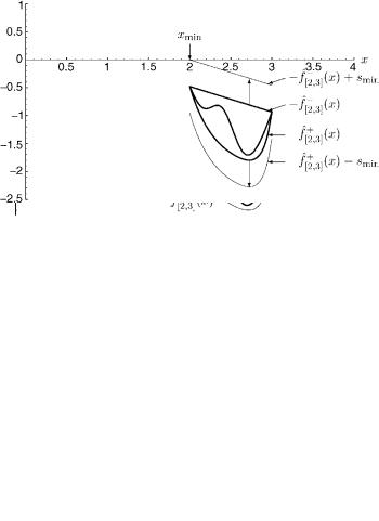
Figure 10. The lower bounding problem for the interval [2, 3] is solved. Note that the convex envelope must be expanded before it touches the x-axis, resulting in a positive value for smin. This interval will be fathomed. (xmin; sminÞ ¼ ð2; þ0:479).

III.STRUCTURE PREDICTION OF POLYPEPTIDES

A.Structure Prediction of Oligopeptides

The use of computational techniques and simulations in addressing the protein folding problem became possible through the introduction of qualitative and quantitative methods for modeling these systems. Given a sufficiently accurate

description of the intramolecular forces, it is in principle possible to predict the folded conformation by optimization. In our work, we have focused not only on the development of global optimization methods, but also on the verification of energy modeling techniques.

In the area of energy modeling, our work has involved the investigation of numerous detailed representations of protein systems. In addition to the traditional all-atom potential energy models, our work has explored the effects of solvation contributions. In fact, although the problem of considering solvation effects in global conformational energy searches has been made tractable by the development of implicit solvation models, results for such formulations are essentially nonexistent, and those that have appeared are for limited searches only. In our work, both solvent accessible area and volume effects have been considered in the context of global searches for oligopeptides. In addition, we have examined the effects of several parameterizations for these models and have been able to identify those that provide the best correspondence between computational and experimental results.

1.Potential Energy Models

There are a number of approaches that may be used to model protein interaction energies. In reality, the dynamics of atoms are governed by the quantum theory of their participating electrons. Using the Born–Oppenheimer approximation, one can determine the energy for fixed atomic nuclei from the smallest eigenvalue of the Hamiltonian of the electron system. These approximations and their derivatives are calculated using ab initio methods. However, due to their computational complexity, such calculations are limited to extremely small molecules. Less detailed, semiempirical methods are based on all atom representations of the peptide. In general, these models, also known as force fields, are expressed as summations of empirically derived potential functions, with the mathematical form of individual energy terms based on the phenomenological nature of that term. Other simplified models have been used to reduce the degrees of freedom associated with the conformational energy expressions.

A number of empirically based molecular mechanics models have been developed for protein systems, including AMBER [29–31], CHARMM [32], DISCOVER [33], ECEPP [34–36], ECEPP/2 [37], ECEPP/3 [38], ENCAD [39,40], GROMOS [41], MM2 [42], and MM3 [43–45]. A general total energy equation, such as Eq. (23), includes terms for bond stretching (Ebond), angle bending (Eangle), torsion (Etor), nonbonded (Enb) and coupled (Ecross) interactions.

deterministic global optimization and ab initio approaches 289

Bond stretching and angle bending energies are included in those force fields that allow flexible geometries. A simple representation for both terms is based on the harmonic approximation, which corresponds to the classical description of the movement of a spring (by Hooke’s law). The simplest approach, based on the fact that most bonds are near the minimum of their respective energy well, employs a quadratic term to model bond stretching and angle bending energies, as shown in Eqs. (24) and (25):

These equations act as penalty functions to force bond distances and bond angles, l and y, to reference bond lengths and distances, l0 and y0, whose values depend on the specific atoms involved. In actuality, these energy terms are more complicated. For bond energies cubic terms are often introduced, and angle energy terms usually include higher power expansions.

Torsional terms are used to describe the internal rotation energy of torsion angles, which exist between all atoms with a 1–4 relationship (separated by two other atoms). For rigid geometry force fields, these torsion angles can be used to define a set of independent variables that effectively describe any protein conformation. This approximately reduces the number of variables by a factor of 10 over those force fields that use a Cartesian coordinate system to describe flexible molecular geometries. In addition, bond and angle energies can be neglected for rigid geometry force fields. The torsion energy expression is typically represented by a Fourier series expansion that, as shown in Eq. (26), includes three terms:

The parameters involved in this expansion—namely E1, E2, and E3—are torsional barriers that are usually specified for the pair of atoms around which the torsion occurs. Each term can be interpreted physically. The 1 x (cos f) symmetry term accounts for those nonbonded interactions not included in general nonbonded terms. The 2 x (cos 2f) symmetry term is related to the interactions of orbitals, while the 3 x (cos 3f) symmetry term describes steric contributions.

Nonbonded energy terms attempt to model electrostatic and van der Waals interactions between those atoms that are not connected to each other or through a common atom. Typically, a Coulombic term is used to represent electrostatic

Here Qi and Qj represent the two point charges, while Rij equals the distances between these two points. In some force fields, Coulombic interactions are modified by changing the dependence of the dielectric constant, E. In general, van der Waals interactions are modeled using a 6–12 Lennard-Jones potential energy term. This expression, shown in Eq. (28), consists of a repulsion and attraction term.

The energy minimum for a given atomic pair is described by the potential depth, Eij, and position, Rij. Other force fields model van der Waals interactions using a modified Hill equation, which replaces the twelfth power term in Eq. (28) with an exponential term [42,43]. Different approaches are also used to describe nonbonded interactions between those atoms that may form hydrogen bonds. Some force fields model these interactions using only Coulombic terms, whereas other force fields employ special functions, such as a modified 10–12 Lennard- Jones-type potential term [46], as shown in Eq. (29).

The cross term, shown in Eq. (23), accounts for interactions due to the inherent coupling between bonds, angles and torsions. Generally, these terms are small, and in many force fields they are neglected. Correction terms, which vary for each force field, are also typically added to the general energy equation. For example, the formation of disulfide bridges can be enforced by adding a penalty term to constrain the values of specified bond angles and bond lengths. Correction terms have also been used to adjust conformational energies according to the configurations of proline and hydroxyproline residues [38].

For a significant portion of this work, the ECEPP/3 (Empirical Conformational Energy Program for Peptides) [38] potential model is utilized. In this force field, it is assumed that the covalent bond lengths and bond angles are fixed at their equilibrium values. Then, the conformation is only a function of

deterministic global optimization and ab initio approaches 291

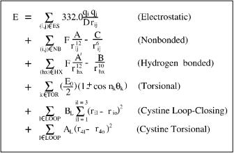
the independent torsional angles of the system, also known as dihedral angles. The total conformational energy is calculated as the sum of the electrostatic, nonbonded, hydrogen bonded, and torsional contributions. There is also a pseudopotential for loop closing if the polypeptide contains two or more sulfurcontaining residues. More recent work includes a revised treatment of prolyl and hydroxyprolyl residues [38]. For each prolyl or hydroxyprolyl residue contained in the polypeptide a fixed internal conformational energy for the pyrolidine ring is added. The main energy contributions (electrostatic, nonbonded, hydrogen bonded) are computed as the sum of terms for each atom pair (i; j) whose interatomic distance is a function of at least one dihedral angle. The general potential energy terms of ECEPP/3 are shown in Fig. 11, while the development of the appropriate parameters is discussed and reported elsewhere [38].

2.Solvation Energy Models

Solvation contributions are generally believed to be a significant force in stabilizing the native conformations of proteins. Explicit methods can be used to include solvation effects by actually surrounding the polypeptide with solvent

Figure 11. Potential energy terms in ECEPP/3 force field. rij refers to the interatomic distance of the atomic pair (ij). Qi and Qj are dipole parameters for the respective atoms, in which the dielectric constant of 2 has been incorporated. Fij is set equal to 0.5 for 1–4 interactions and equal to 1.0 for 1–5 and higher interactions. Aij, Cij, A0ij, and Bij are nonbonded and hydrogen bonded parameters specific to the atomic pair. Eo;k and Eo;l are parameters corresponding to torsional barrier energies for a given dihedral angle. yk represents any dihedral angle. ck takes the values 1, 1, and nk refers to the symmetry type for the particular dihedral angle. The cystine loop-closing term is calculated as a penalty term of three distances involved in loop-closing, where ril represents the actual distance and rio represents the required distance. Bi, the penalty parameter, is set equal to 100. Finally, Ep is a fixed internal energy that is added for each proline residue in the protein. Energy

˚

units are kcal/mol and distance units are A.

molecules and calculating solvent–peptide and solvent–solvent interactions. Although these methods are conceptually simple, explicit inclusion of solvent molecules greatly increases the computational time needed to simulate the polypeptide system. Therefore, most simulations of this type are limited to restricted conformational searches. In addition, it is difficult to quantify the effect of hydrophobic interactions that result from the ordering of water molecules.

Methods for estimating solvent free energies have also been developed using both integral equations and continuum models. Integral equation methods can be used to evaluate solvent structure and thermodynamic properties. Typically, molecular dynamics or Monte Carlo simulations are used to calculate ensemble averages from which free energy differences can be obtained. A number of methods have been proposed to estimate these solvation free energies from simulations based on molecular dynamics and Monte Carlo averages [47–49]. The integral equation method has also been used to analyze the solvent structure of a protein system [50]. In contrast, continuum models use a simplified representation of the solvent environment by neglecting the molecular nature of the water molecules. Calculations of solvation free energies using electrostatic continuum models rely on numerical solutions to the Poisson–Boltzmann equation from which dielectric and ionic strength effects are obtained [51]. Other continuum models estimate free energies of solvation as a function of surface areas and volumes.

In this work, solvation contributions are included implicitly using empirical correlations with both surface area [52] and volume [53]. The main assumption of these models is that, for each functional group of the peptide, a hydration free energy can be calculated from an averaged free energy of interaction of the group with a layer of solvent known as the hydration shell. In addition, the total free energy of hydration is expressed as a sum of the free energies of hydration for each of the functional groups of the peptide; that is, an additive relationship is assumed.

Accessible surface area methods assume that the free energy of hydration is proportional to the solvent-accessible surface area of the peptide, as described by the following equation:

i¼1

In Eq. (30), an additive relationship for N individual functional groups is assumed. (Ai) represents the solvent-accessible surface area for the functional group, and (si) is an empirically derived free energy density parameter.

There are a number of ways to define the surface of a peptide. In developing these surfaces the peptide is represented by a union of spheres, with the radii of

deterministic global optimization and ab initio approaches 293

the spheres set by the van der Waals radii of the constituent atoms. A spherical test probe is then rolled over these spheres, thereby tracing out a surface. The molecular surface is set by direct contact between the probe sphere and the peptide spheres. In areas where the probe cannot make direct contact, the closest part of the probe is used. The solvent-accessible surface is defined by the surface traced by the center of the probe as the probe rolls over the peptide spheres. These areas depend on the radius of the probe sphere; when this radius is set to zero, both the molecular and solvent–accessible surface areas become the van der Waals surface of the peptide.

Solvent-accessible surface areas are calculated using the MSEED [52] program, which employs algorithms developed by Connolly [54]. MSEED eliminates many unnecessary computations by considering only those convex faces that are on the accessible surface. Rigorous implementation of Connolly’s method requires the calculation of interior surface areas, which are ultimately found to be zero. A full description of the MSEED algorithm is given elsewhere [52]. A number of other methods for calculating surface areas are also available [55–57].

One potential problem that may arise when calculating accessible surface areas is the appearance of gradient discontinuities. This may occur when a new vertex or edge appears on the surface. If the discontinuity is large, minimization techniques requiring gradients may fail to converge to the local minimum conformation. A complete analysis of all situations for which the gradient of the molecular surface area becomes discontinuous has been reported [58].

Once the solvent–accessible surface areas have been calculated, these values must be multiplied by the appropriate (si) parameters as shown in Eq. (30). A variety of parameter sets have been developed to model the transfer of atoms from a gaseous to a hydrated environment. The parameter values for the five ASP sets used in this study are given in Table I.

The ASP sets WE1 and WE2, are taken from Table 3 of Ref. 59. These parameters are both derived from Wolfenden’s measured free energies of transfer of amino acid side-chain analogs from vapor to water [60]. Both sets have been adjusted to correct for entropy of mixing effects based on solute and solvent size differences [61,62], although the applicability of these corrections has been criticized [63,64]. The parameters for these two sets are negative for all atoms excluding carbon. Qualitatively, this means that the nitrogen, oxygen, and sulfur atoms are considered hydrophilic; that is, they favor solvent exposure. Comparatively, the WE1 and WE2 parameters are similar, with the largest relative difference being a 3 : 1 ratio (WE1 : WE2) for the sC parameter. Therefore, the hydrophobic character of these carbon atoms is stronger for the WE1 ASP set.

The OONS parameter set has been specifically developed to supplement the ECEPP/2 force field [65]. These parameters were derived by a least squares

TABLE I

Free Energy Density of Solvation Parameters for the ASP Set Employed with the Solvent-Accessible Surface Area Modela

aThe first column describes the atom type, whereas the remaining columns provide the solvation

˚ 2

parameters in cal/(mol A ) for the corresponding ASP set.

fitting to experimental free energies of gas to water transfer of small aliphatic and aromatic molecules. The most significant difference from the two previous ASP sets is a substantial increase in hydrophobic character for carboxyl (carbonyl) carbon atoms, which corresponds to a hundredfold increase when compared to the same WE2 parameter. In addition, the free energy parameter becomes negative for aromatic carbons, which indicates a hydrophilic tendency. The threefold decrease of the OONS values for carboxyl (carbonyl) and charged oxygen atom parameters, as compared to both the WE1 and WE2 ASP sets, is also significant.

Unlike the aforementioned models, the SCKS ASP set is not directly based on experimental free energies [66]. Instead, it is an optimized parameter set developed to complement the CHARMM [32] molecular mechanics force field. Specifically, through the use of experimental and molecular dynamics information, the relative weightings of solvation parameters were refined to provide the best correspondence between minimized and experimental structures. In comparing the individual free energy parameters, it is evident that the hydrophobic character of the carbon atoms is increased approximately threeand eightfold over the WE1 and WE2 values, respectively. In contrast, the uncharged oxygen and nitrogen atom parameters are 6.5 times smaller (less hydrophilic) than those for the WE1 and WE2 ASP sets. This decrease does not apply to charged oxygen and nitrogen atoms, which possess extremely hydrophilic values.

The JRF ASP set was derived from NMR studies of low energy solvated configurations of 13 tetrapeptides [67]. This represents an important difference from other derivations because actual peptides, rather than simple model compounds, were used to develop the JRF parameters. An ensemble of lowenergy structures for these tetrapeptides was also produced using the ECEPP/2

deterministic global optimization and ab initio approaches 295

potential function. Then, a nonlinear least-squares system was optimized for the best set of atomic solvation parameters. Although the parameters for oxygen, nitrogen, and sulfur atoms are negative, their large absolute values indicate much larger hydrophilicities than corresponding atoms of any other ASP set. In addition, both the carboxyl (carbonyl) and aromatic carbon atoms possess strong hydrophilic parameters, which contradicts other free energy parameter values for these atoms. The single positive value belongs to the aliphatic carbon atom type, which, although larger than any other parameter for this atom type, possesses the smallest magnitude for the JRF ASP set. Furthermore, because it was developed from minimum energy conformations of peptides, the JRF ASP set has been shown to produce undesirable perturbations during local minimizations if the solvation energy contributions are added at every iteration. Therefore, unlike the aforementioned ASP sets, the JRF solvation energy effects are only included at local minimum conformations.

For volume shell models, the free energy of hydration is assumed to be proportional to the water-accessible volume of a hydration layer surrounding the peptide. This can be represented in the form

i¼1

An additive relationship for the N individual atoms of the peptide is assumed, and (VHSi) represents the solvent-accessible volume of hydration shell for each atom i that is exposed to water. The (di) parameters are empirically determined free energy of hydration densities for these atoms.

The hydration shell is defined by the volume inside a sphere of radius Rhi but outside a sphere of radius Rvi , with both radii centered on atom i. The larger radius, Rhi , corresponds to the radius of the first hydration shell of atom i, while Rvi is equal to the van der Waals radius. In order to calculate (VHSi), the volume of a collection of overlapping hard spheres must be computed using:

In Eq. (32), Si signifies the volume of a single sphere, while Dij, Tijk and Qijkl represent the volume of intersection of two, three, and four spheres, respectively. This is sufficient because all higher-order overlaps can be decomposed into the three types of intersections included in Eq. (32). Therefore, the solventaccessible volume of hydration can be written as