Friesner R.A. (ed.) - Advances in chemical physics, computational methods for protein folding (2002)(en)

TABLE VII

Comparison of Rankings for PDB Secondary Structure and DSSP Secondary Structure for Several Cases from the Test Set

typically thousands of energy units. This is in sharp contrast to the results obtained with our previous tertiary folding potential, which routinely generated energy gaps between misfolded and native-like structures that were 5–10 times larger than those seen here.

D.Effects of Secondary Structure Definition and Truncation of Terminal Loops

The results presented above employ PDB-defined secondary structure and in some cases involve truncation of terminal loops, primarily carried out here to facilitate direct comparisons with the results of Ref. 2. However, the process of defining secondary structure even with X-ray crystallographic or NMR coordinates in hand is not entirely unambiguous, and the effects of terminal loops could be favorable or unfavorable. To examine these issues, we selected several proteins in Table V for which the results with the new potential appeared less accurate than would have been expected given the difficulty of the case being considered. Table VII presents results for these selected cases, listing the protein and identifying what experiments were carried out. Most of the cases examined are mixed a/b because these displayed the most significant problems. It can be seen that in some cases the use of a different secondary structure definition (e.g., DSSP rather than PDB) and the inclusion or deletion of a terminal loop has a substantial effect on the ranking of low RMSD structures. Clearly, more work needs to be done in understanding these effects.

E.Effects of Using Ideal Rather than PDB-Derived Three-Dimensional

Topologies for Secondary Structure Elements

Having established that our new size-dependent potential is quite effective for generating low-resolution structures of proteins below 100 residues using secondary structure derived from PDB coordinates, we next ask what the effect is of using ideal torsional angles for helices and strands as opposed to PDB-derived

246 volker a. eyrich, richard a. friesner, and daron m. standley

torsion angles. Tables V and VIc summarize results for the entire test set of proteins utilizing ideal secondary structure elements. The results are surprisingly good; while there are certainly cases in which quantitative degradation of the rank of the best low-RMSD structure occurs (particularly with a/b-proteins—for example, the proteins 2fdn, 1fwp, and 5pti), in general the simulations are able to find such structures successfully and to rank them reasonably well in terms of total energy. Even in the case of 5pti, where there is severe distortion of the b- strands in the native structure, the use of ideal strands produces reasonable results. While incorporation of strand distortion is possible in our methodology [4], the reasonable predictive capability using ideal elements is likely to save considerable computational effort because one can carry out such simulations initially and then use the results as a starting point from which to incorporate distortions and other detailed effects.

IV. USE OF PREDICTED RATHER THAN PDB-DERIVED

SECONDARY STRUCTURE ELEMENTS

A.Overview

Secondary structure prediction methods, while they have improved significantly over the past decade (principally via the use of multiple sequence analysis), still have nontrivial error rates. The best method at present appears to be the PSIPRED approach developed by Jones [26], which is claimed to achieve an accuracy between 76% and 78% on a reasonably large training set (it also outperformed other methods in the CASP3 contest). This level of reliability appears to be sufficient for low-resolution ab initio structure prediction and suggested to us that it was now worth experimenting with tertiary folding calculations based entirely on predicted, rather than PDB-derived, secondary structure [27–32]. Using servers set up on the World Wide Web, we are able to obtain predictions from PSIPRED and other secondary structure prediction algorithms for proteins in our test set. We have obtained results from a variety of servers to see what happens in cases where their predictions disagree; it is likely that ab initio prediction will involve trying a number of secondary structures, because in some cases the tertiary fold will be critical in selecting among plausible secondary structures predicted exclusively from sequence data.

Our calculations in this section endeavor to answer the following questions:

1.Can we for some percentage of cases make a successful ab initio prediction? We explore two different approaches below.

2.What are the effects of small errors in secondary structure—for example, elimination or addition of small elements, incorrect lengths of major elements and so on?

3.What is the impact of a major error—for example, replacing a long helix by a similar strand or missing an important loop?

In the present chapter, we have chosen to focus our ab initio prediction efforts primarily on a-helical proteins, although one mixed a/b-protein is also examined. The ab initio prediction calculations presented below are considerably more computationally intensive than those using PDB-derived secondary structure, because we have investigated a substantial number of secondary structure predictions for each protein. By studying helical systems intensively, we are able to draw conclusions concerning the necessary and sufficient conditions for success for such systems from a significant database of results. In addition to the a-helical proteins in the 50to 100-residue range from the data set above, we also include two helical proteins from the CASP3 prediction contest. Our results for the CASP3 test cases are similar to those from the PDBderived test suite.

B.Secondary Structure Prediction Methods

We use the following secondary structure prediction methods in our ab initio predictions:

*PSIPRED [26]: A two-stage neural network that predicts protein secondary structure based on the position specific scoring matrices generated by PSI-BLAST (available at http: //insulin:brunel:ac:uk/psipred/Þ. Average three-state prediction accuracy is between 76.5% and 78.3%. Currently the most accurate method.

*PhD [33,34]: Secondary structure is predicted by a system of neural networks (available at http: //cubic:bioc:columbia:edu/pp/Þ. Overall threestate prediction accuracy is 72.1%. The default secondary structure prediction settings were used in all predictions.

*JPRED [35,36]: A methodology that combines a total of six secondary structure predictions into one consensus prediction (available at http:// jura.ebi.ac.uk:8888/ at the time of this writing). Average ‘‘real world’’ accuracy is 72.9%. Note that the PhD predictions generated by JPRED differ from the original PhD predictions (denoted: orig_phd) mentioned above. In addition to using the consensus prediction, we also report results for the six individual prediction methods included in the JPRED server.

By default, secondary structure prediction accuracies reported here are determined with DSSP as the reference (for details see Ref. 26). The secondary structure assignments used in the actual calculation differ from the original predictions in that helices and strands of less than three residues are eliminated. N- and C-terminal loops are deleted.

248 volker a. eyrich, richard a. friesner, and daron m. standley

C.Simulation Protocols

The amino acid sequence of the target represents the only input data for our methodology. We do not carry out explicit database searches (i.e., threading) of any sort. Secondary structure predictions from the sources listed above are parsed and used directly in the structure predictions. In the case of JPRED we examine individually the results of all predictions that contribute to the consensus prediction (DSC [37], PhD [33,34], PREDATOR [38,39], NNSSP [40], Mulpred, and Zpred [41]). Because we do not assume any knowledge of approximate radius of gyration of the target, which is important for the selection of the correct potential energy parameters, we predict the radius of gyration via a simple formula [22] and use this prediction to assign the size bin for the tertiary folding simulation.

The first stage of our prediction algorithm applies the MCM-based approach described above to each of the nine secondary structure predictions for each target. Simulations are usually carried out on two to four nodes of a multiprocessor machine and take between 12 and 24 hours depending on protein size. To extract the structurally unique predictions, we apply the clustering algorithm discussed above. Table VIII shows the results of this procedure for the three targets discussed in more detail below. We list results for every secondary structure prediction (unless predictions consist only of loop or coil, in which case we did not believe it worthwhile to carry out the simulation).

Because it is quite possible that simulations utilizing different secondary structure predictions results in very similar representative low energy structures, we apply a second level of filtering which basically tries to eliminate structurally similar predictions and ranks the resulting ‘‘unique’’ predictions on a absolute energy scale. The first step in this process is the determination of the subset of residues common to all predictions (regardless of whether they belong to helices or strands). Secondary structure predictions for which the number of residues included in the simulation is substantially smaller than the average (due

TABLE VIII

Individual Clustering Results for the ab initio prediction Targets Discussed in More Detail in the Text (Stage 1 of the Composite Prediction Method)a

aHere Nres refers to the number of residues actually considered for every prediction. (cons: JPRED consensus prediction; dsc: DSC; mul: MULPRED; nnssp: NNSSP; orig_phd: PhD in its most current implementation; phd: PhD as run by JPRED; pred: PREDATOR; psipred: PSIPRED; zpred: ZPRED). Q3 refers to the three-state accuracy of a given prediction.

250 volker a. eyrich, richard a. friesner, and daron m. standley

to deletion of terminal loops) are not considered at this stage. This set of residues is then extracted from the 50 clusters lowest in energy for every secondary structure prediction, and the energies of the resulting substructures are evaluated. After a second round of clustering, we obtain the final set of clusters (Table IX). At this point the RMSDs with respect to the native structures are reevaluated over the subset of common residues to allow a fair comparison of the tertiary folding results obtained from different secondary structure predictions. We refer to this method below as the composite energy prediction method.

D. Final Rankings of Structures for Fully Ab Initio Predictions

We examine the use of two different approaches for producing fully ab initio predictions for the 22 proteins studied in this section. One approach is simply to use the secondary structure prediction with the highest calibrated prediction— accuracy—in this case, PSIPRED. Results for this approach are summarized in

TABLE IX

Final Clustering Results for the Subset of Common Residues for All Ab Initio Prediction Targets (Stage 2 of the Composite Energy Prediction Method)a

aHere Nres refers to the number of residues for which RMSD and energy are evaluated. We omitted predictions that were too short as compared to all others and the length of the sequence (1eh2: mul; 1jvr: psipred; 1mzm: cons, phd, pred; 1r69: mul, orig_phd, pred; 2ezh: orig_phd).

TABLE X

Individual Clustering Results for All Ab Initio Prediction Targets Using the PSIPRED Secondary Structure Predictionsa

aHere Nres refers to the number of residues actually considered for every prediction.

Table X. As above we list the rank of structures below a certain RMSD cutoff. The second is the composite energy prediction method discussed above. We summarize statistics for the success rate of each of these two approaches on the entire test set and CASP3 prediction targets below.

E.Results

1.Summary and Overall Success of Fully Ab Initio Prediction

We begin by summarizing the results for all of the secondary structure prediction methods (including the composite energy prediction method described above) and all of the target proteins. As in previous sections of this chapter, the ranks of

˚ ˚ ˚

the lowest-energy cluster with RMSDs from the native structure of 4 A, 5 A, 6 A,

˚

and 7 A are reported for both approaches. The first, and most striking, observation is that both approaches provide a surprisingly good success rate for ab initio prediction based on criteria used in CASP3. We have observed that for proteins

˚

in the 50–100 residue range, an RMSD below 7 A typically provides a

252 volker a. eyrich, richard a. friesner, and daron m. standley

qualitatively reasonable folding topology at low resolution. Similar conclusions have been reached by Skolnick and co-workers [42] and by Cohen and Sternberg [43], whose estimates show that the probability of achieving a structure below 6

˚

A RMSD by chance is vanishingly small. Note also that for a significant fraction

˚

of proteins, structures below 6 A are found; at this level, the correspondence with the native structure is quite satisfactory in agreement with the chapters cited above.

Both proposed fully ab initio prediction methods (composite energy method and exclusive use of PSIPRED predictions) yield a number of cases in which a low RMSD structure is ranked first; this would count as a successful prediction under any criterion. Using the assessment criteria of CASP3—that is, a maximum of five predictions—the composite energy method would achieve

˚

an RMSD of less than 7 A in 68% of the cases; there are also four cases where

˚

the RMSD is less than 6 A. Reliance entirely on PSIPRED would lead to an

˚

RMSD under 7 A in 64% of the cases; however, 11 of those would have an

˚

RMSD under 6 A. Thus, the use of the composite energy method appears to succeed slightly more often, however, the use of PSIPRED exclusively generates highly accurate predictions in significantly more cases.

We have employed the protocol described above in a completely automated fashion; but only in an actual blind test can one be sure that the results suffer from no unconscious bias. If these results hold up under truly blind test conditions, this would represent a significant advance in ab initio prediction methodology as judged by other ab initio efforts in CASP3.

While our new potential energy function certainly represents a step forward, there are also obviously areas where more work needs to be done. Primarily, the causes of failure to routinely achieve a low-RMSD structure in the top five predictions in some cases must be analyzed and understood. These failures are thus more interesting at this point than the successes because they point the way to development of an improved methodology. We therefore analyze a number of these cases in detail below so as to reveal the underlying difficulties and directions in which solutions must be developed.

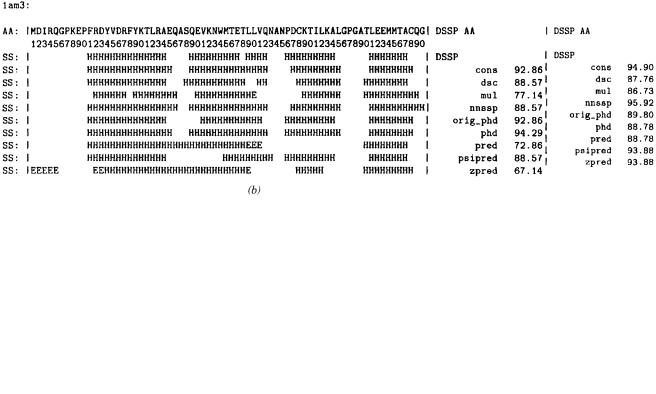
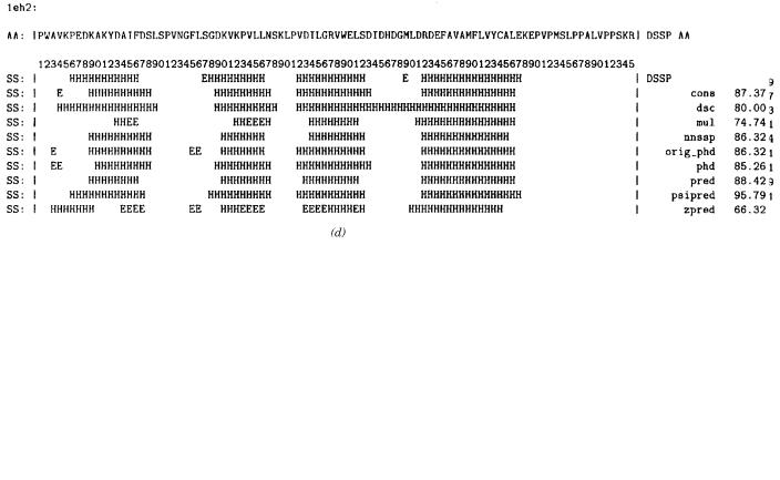
2.Detailed Analysis of Specific Cases

Figure 8 presents the detailed secondary structure predictions for each of the cases that we analyze below. In conjunction with the tertiary folding results summarized in Table VIII, as well as the results using PDB-derived secondary structure presented above, we can extract insight into how various types of errors in secondary structure prediction affect tertiary folding accuracy. Due to the large amount of data, we have selected a subset of interesting examples to analyze in detail, however, the conclusions, summarized in the discussion following consideration of individual examples, reflect an examination of the results for all 22 of the proteins studied.