Baer M., Billing G.D. (eds.) - The role of degenerate states in chemistry (Adv.Chem.Phys. special issue, Wiley, 2002)

125.R. Izzo and M. Klessinger, J. Comput. Chem. 21, 52 (2000).

126.E. Havinga and J. Cornelisse, Pure Appl. Chem. 47, 1 (1976).

127.N. J. Turro, Modern Molecular Photochemistry, Bejamin/Cummings, Menlo Park, CA, 1978.

128.D. I. Schuster, G. Lem, and N. A. Kaprinidis, Chem. Rev. 93, 3 (1991).

129.J. Michl, Photochem. Photobiol. 25, 141 (1977).

130.L. Salem and C. Rowland, Angew. Chem. Int. Ed. Engl. 11, 92 (1972).

131.L. Salem, Science. 191, 822 (1976).

132.J. A. Berson, Acc. Chem. Res. 11, 466 (1978).

133.J. Michl, Mol. Photochem. 4, 243–257 (1972).

134.J. Michl, Top. Curr. Chem. 46, 1 (1974).

135. J. Michl, in ‘‘Photochemical Reactions: Correlation Diagrams and Energy Barriers,’’ G. Klopman, ed., Chemical Reactivity and Reaction Paths, John Wiley & Sons, Inc., New York, 1974.

136.J. Michl and V. Bonacic-Koutecky, Electronic Aspects of Organic Photochemistry, John Wiley & sons; Inc. New York, 1990.

137.L. Salem, J. Am. Chem. Soc. 96, 3486 (1974).

138.R. McWeeny and B. T. Sutcliffe, Methods of Molecular Quantum Mechanics, Academic Press, 1969, Chap. 6.

139.H. Eyring, J. Walter, and G. E. Kimball, Quantum Chemistry, John Wiley & Sons, Inc., New York, 1944, Chap. 13.

140.L. Pauling, J. Chem. Phys. 1, 280 (1933).

I.INTRODUCTION

The introduction of the conventional Born–Oppenheimer (BO) approximation introduces the concept of electronic potential energy surface (PES), which lays the foundation of the majority of our concepts about molecular systems. However, the crossing of two adiabatic PES is also a consequence of such an adiabatic approximation. There has been much research done in an attempt to remove the singularity brought about by this crossing of multi-dimensional surfaces, namely, the conical intersections. Recently, characterization of conical intersection in molecules and the role played by conical intersection in femtosecond processes have attracted considerable attention [1–4]. The conical intersection is conventionally determined by the use of the adiabatic approximation. There are a number of so-called adiabatic approximations for the time-independent quantum mechanical treatment of molecules [5–13]. The most prominent of them are the BO approximation and the Born–Huang (BH) approximation. This latter name of BH approximation was suggested by Ballhausen and Hansen, but the theory was actually formulated by Born himself. It has also been described as the BO correction, the variational BO approximation and the Born–Handy formula. First, these approximations all start with the separation of the total molecular Hamiltonian into terms of different magnitude. Second, it is very common that, while trying to sort out terms of different magnitude, attempts were given to argue that the crossing terms coupling the momenta of the various atoms in the molecule are negligible after proper transformations. Ballhausen and Hansen made a very instructive comment saying that [8] ‘‘The effect of these cross-terms is to correlate the internal motion, so to speak, in such a way that the linear momentum as well as the angular momentum of the entire molecule stay constant.’’ It is worth noting that actually these cross-terms are not only crucial for keeping the momentum constant, but also are important for keeping the energy constant. This point has not been proved rigorously, but it can be understood by noticing that the concept of electronic potential energy is a direct consequence of the adiabatic approximation. The negligence of the nuclear kinetic energy term and the fixation of the nuclear coordinates (and thus the frozening of the dependence of the cross-terms on the nuclear coordinates) are the causes of the dependence of the electronic energy on the nuclear configuration.

The separation of the electronic degrees of freedom from nuclear motions through adiabatic approximation has brought success to the ab initio quantum chemistry computations, but it is also the reason why we are confronted with the very difficult problem of potential energy crossing, in particular, the conical intersections. There may be other approaches, however, in which the energies of the states depend neither functionally nor parametrically on the nuclear configuration, and hence no crossing of energy levels may occur. If an approach like this can

be developed, and if it is computationally tractable, then it may be a good method complement to the contemporary quantum chemistry packages for treating the cases in which potential energy surfaces crossing may happen in the traditional approach.

An alternative approximation scheme, also proposed by Born and Oppenheimer [5–7], employed the straightforward perturbation method. To tell the difference between these two different BO approximation, we call the latter the crude BOA (CBOA). A main purpose of this chapter is to study the original BO approximation, which is often referred to as the crude BO approximation and to develop this approximation into a practical method for computing potential energy surfaces of molecules.

In this chapter, we demonstrate the approach of the CBOA, and show that to carry out different orders of perturbation, the ability to calculate the matrix elements of the derivatives of Coulomb interaction with respect to nuclear coordinates is essential. Therefore, we studied the case of the diatomic molecule, and here we demonstrate the basic skill of computing the relevant matrix elements in Gaussian basis sets. The formulas for diatomic molecules, up to the second derivatives of the Coulomb interaction, are shown here to demonstrate that some basic techniques can be developed to carry out the calculation of the matrix elements of even higher derivatives. The formulas obtained may be complicated. First, they are shown to be nonsingular. Second, the Gaussian basis set with angular momentum can be dealt with in similar ways. Third, they are expressed as multiple finite sums of certain simple functions, of order up to the angular momentum of the basis functions, and thus they can be computed efficiently and accurately. We show the application of this approach on the H2 molecule. The calculated equilibrium position and force constant seem to be reasonable. To obtain more reliable results, we have to employ a larger basis set to higher orders of perturbation to calculate the equilibrium geometry and wave functions.

II.CRUDE BORN–OPPENHEIMER APPROXIMATION

The theory discussed in this section is based on the work of Born and others [5,7]. However, some of the approaches that are not suitable for our need are modified, and proper notations are adopted accordingly.

For a molecular system, we shall separate the total Hamiltonian into three parts:

^

The T operators are the usual kinetic energy operators, and the potential energy Vðr; RÞ includes all of the Coulomb interactions:

Let us consider the simplified Hamiltonian in which the nuclear kinetic energy term is neglected. This also implies that the nuclei are fixed at a certain configuration, and the Hamiltonian describes only the electronic degrees of freedom. This electronic Hamiltonian is

Note that the last term in expression (2) of V does not depend on electronic

^

coordinates, and therefore it may be neglected in H0. The adiabatic Hamiltonian still depends parametrically on R, and so is the electronic wave funcion jfi. If we expand the nuclear coordinates or some of the nuclear coordinates with respect to a given configuration, that is, if we define

where k is a natural perturbation parameter that will be described later, then we shall expand the Hamiltonian in powers of k as

.

.

.

Note that the electronic kinetic energy operator does not depend on the nuclear configuration explicitly. Therefore, we can conclude that

.

.

.

In the following, it shall always be assumed that the zeroth-order solution is known, that is, we have a complete set of eigenvalues and wave functions, labeled by the electronic quantum number n, which satisfy

Next, we shall consider how the nuclear kinetic energy is taken into consideration perturbatively. The natural perturbation index k is chosen to be

where m is the electron mass and M0 is some quantity to do with the mass of

^

nuclei. In rectangular coordinates, TN can be written as

Since the nuclear coordinates are expanded according to Eq. (5), we can write the derivatives in the kinetic energy expression as

^ ð2Þ

where in H1 , all of the derivatives with respect to nuclear coordinates R are replaced by derivatives with respect to R , while the rest of the expression remains unchanged. In this case, the total Hamiltonian can be expanded into power series of k as

This requires that the initially chosen R0 be the equilibrium configuration of this electronic level. Also, we reach the conclusion that the wave function will be of the form

Furthermore, we obtain the equation of motion of the zeroth-order nuclear wave function:

We can only determine Enð2Þ and jwðn0Þi up to now. Later, we shall demonstrate that this equation is just the equations of motion of harmonic nuclear vibrations. The set of eigenstates of Eq. (43) can be written as fjwnvig, symbolizing that they are the vibrational modes of the nth electronic level, where v ¼ ðv1; v2; . . . ; vN Þ if R is N dimensional, and vi is the vibrational quantum number of the ith mode.

In the third-order approximation, the equations are

The electronic wave functions and potential energy can be determined in ways similar to those done in the first and second order. Here we wish to emphasize that, the full wave function in this order is

This means that the electronic and nuclear wave functions cannot be separated anymore, and therefore the adiabatic approximation cannot be applied beyond the second-order perturbation.

In the following, we shall demonstrate techniques for calculating the electronic potential energy terms up to the second order. For simplicity, we shall study the case of H2 molecule, the simplest multi-electron diatomic molecule.

III.HYDROGEN MOLECULE: HAMILTONIAN

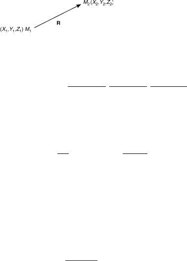
Consider a diatomic molecule as shown in Figure 1. The nuclear kinetic energy is expressed as

Figure 1. A model two-atom molecule.

where R0 is the coordinate of the center of mass, one can rewrite the nuclear kinetic energy:

Here, we have defined