

Baer M., Billing G.D. (eds.) - The role of degenerate states in chemistry (Adv.Chem.Phys. special issue, Wiley, 2002)
.pdfapplying direct molecular dynamics to non-adiabatic systems 393
torsional motion labeled Q5. Four Ag modes are present, which may have firstorder expansion coefficients on the diagonal of the diabatic potential matrix. After the parameters for the Taylor expansions are fitted to quantum chemical calculations [170,190], it is found that only one symmetric mode, the central C C stretch Q14, has a significant linear coupling constant, k. Thus this system can be well described considering only two modes, Q5 and Q14.
In Figure 7a the diabatic surfaces are plotted, that is, the on-diagonal functions from the potential matrix. These diabatic PES are interlocking harmonic wells, and they would be the adiabatic surfaces in the absence of nonadiabatic coupling. Compared to the neutral ground-state surface, the two minima have been shifted along the totally symmetric coordinate. Now, including the off-diagonal vibronic coupling term, the adiabatic surfaces change dramatically. They are plotted in Figure 7b, where the PES has been cut away to reveal the conical intersection between the two surfaces. Note also that the minima are now shifted significantly along the torsional, Q5, axis. This deformation away from the D2h symmetry is thus due to non-adiabatic effects.
|
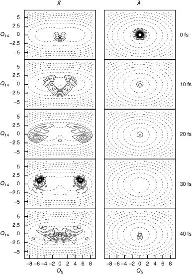
In Section II.B, the molecular dynamics was examined after excitation to the |
~ |
~ |
A state ignoring the coupling to the X state, that is, the PES in Figure 4 is the
higher energy diabatic well in Figure 7a. Figure 8 shows the same dynamics
~
including the non-adiabatic coupling. Starting in the A state, the wavepacket is
~
seen to transfer very fast to the lower X state, with the transfer taking place around the intersection point. Notice the complicated dynamics of the wavepacket on the lower surface that runs around the double well. After 40 fs, the wavepacket has returned to the intersection point, and a small recrossing is seen to the upper surface.
The vibronic coupling model has been applied to a number of molecular systems, and used to evaluate the behavior of wavepackets over coupled surfaces [191]. Recent examples are the radical cation of allene [192,193], and benzene [194] (for further examples see references cited therein). It has also been used to explain the lack of structure in the S2 band of the pyrazine absorption spectrum [109,173,174,195], and recently to study the photoisomerization of retinal [196].
IV. NON-ADIABATIC MOLECULAR DYNAMICS
As shown above in Section III.A, the use of wavepacket dynamics to study nonadiabatic systems is a trivial extension of the methods described for adiabatic systems in Section II.B. The equations of motion have the same form, but now there is a wavepacket for each electronic state. The motions of these packets are then coupled by the non-adiabatic terms in the Hamiltonian operator matrix elements. In contrast, the methods in Section II that use trajectories in phase space to represent the time evolution of the nuclear wave function cannot be
applying direct molecular dynamics to non-adiabatic systems 395
easily extended to systems that evolve in a manifold of coupled electronic states. For this, we need mixed methods that treat the electronic degrees of freedom using quantum mechanics, while using the classical or semiclassical methods for the nuclei.
The standard semiclassical methods are surface hopping and Ehrenfest dynamics (also known as the classical path (CP) method [197]), and they will be outlined below. More details and comparisons can be found in [30–32]. The multiple spawning method, based on Gaussian wavepacket propagation, is also outlined below. See [1] for further information on both quantum and semiclassical non-adiabatic dynamics methods.
A.Ehrenfest Dynamics
Both the BO dynamics and Gaussian wavepacket methods described above in Section II separate the nuclear and electronic motion at the outset, and use the concept of potential energy surfaces. In what is generally known as the Ehrenfest dynamics method, the picture is still of semiclassical nuclei and quantum mechanical electrons, but in a fundamentally different approach the electronic wave function is propagated at the same time as the pseudoparticles. These are driven by standard classical equations of motion, with the force provided by an instantaneous potential energy function
_ |
Pa |
|
ð88Þ |
||
Ra ¼ ma |
|||||
_ |
|
|
q |
|
ð89Þ |
Pa ¼ qRa hcðr; tÞjHelðRÞjcðr; tÞi |
|||||
and a time-dependent Schro¨dinger-like equation for the electronic wave function
_ |
ð90Þ |
icðr; tÞ ¼ HelðRÞcðr; tÞ |
Note that the Hamiltonian is time dependent due to the time dependence of R. There is also a phase corresponding to each trajectory
_ |
ð91Þ |
iA ¼ hcðr; tÞjHelðRÞjcðr; tÞiA |
Details of the derivation of these equations are given in Appendix C.
The expression for the force on the nuclei, Eq. (89), has the same form as the BO force Eq. (16), but the wave function here is the time-dependent one. As can be shown by perturbation theory, in the limit that the nuclei move very slowly compared to the electrons, and if only one electronic state is involved, the two expressions for the wave function become equivalent. This can be shown by comparing the time-independent equation for the eigenfunction of Hel at time t


applying direct molecular dynamics to non-adiabatic systems 397
depend on R, the Ehrenfest force in Eq. (89) can be evaluated using the wave function Eq. (92) by
|
|
|
X |
|
|
|
cjad |
|
|
|
|
cðtÞ ¼ |
|
|
|
ð95Þ |
|
|
cðtÞ |
$Hel |
ci cj ciad |
$Hel |
||||
ij
Note that the exact adiabatic functions are used on the right-hand side, which in practical calculations must be evaluated by the full derivative on the left of Eq. (24) rather than the Hellmann–Feynman forces. This form has the advantage that the R dependence of the coefficients, ci, does not have to be considered. Using the relationship Eq. (78) for the off-diagonal matrix elements of the righthand side then leads directly to
P_ ¼ Xjcij2 |
$Vi X ci cj Vj Vi dij |
ð96Þ |
i |
i¼6 j |
|
The first term on the right of this equation is the average force from the adiabatic potential energy surfaces. The second term is a force due to the non-adiabatic coupling. This mean-field potential is inherent in the method. That it leads to practical problems can be seen by considering the case of a bound state coupled to a dissociative state. Non-adiabatic forces will cause the dissociative state to be populated. The mean-field force, however, gives a bound component to the experienced potential, which may prevent the trajectory from reaching the dissociative region. A discussion of this incorrect behavior is found in [199].
B.Trajectory Surface Hopping
The simplest way to add a non-adiabatic correction to the classical BO dynamics method outlined above in Section II.B is to use what is known as surface hopping. First introduced on an intuitive basis by Bjerre and Nikitin [200] and Tully and Preston [201], a number of variations have been developed [202–205], and are reviewed in [28,206]. Reference [204] also includes technical details of practical algorithms. These methods all use standard classical trajectories that use the hopping procedure to sample the different states, and so add non-adiabatic effects. A different scheme was introduced by Miller and George [207] which, although based on the same ideas, uses complex coordinates and momenta.
The motivation comes from the early work of Landau [208], Zener [209], and Stueckelberg [210]. The Landau–Zener model is for a classical particle moving on two coupled 1D PES. If the diabatic states cross so that the energy gap is linear with time, and the velocity of the particle is constant through the nonadiabatic region, then the probability of changing adiabatic states is
2pH122 |
ð97Þ |
P2!1 ¼ exp hvjF1 F2j |

398 |
g. a. worth and m. a. robb |
where v is the velocity of the particle, Fi ¼ dHii=dR is the force on the ith diabatic surface, and Hij is the Hamiltonian matrix elements in the diabatic basis. All quantities are evaluated at the crossing point. The result is that for high velocity, or small diabatic coupling, the probability of staying on a diabatic surface (changing adiabatic state) approaches 1. The opposite happens for low velocities and strong couplings.
Stueckelberg derived a similar formula, but assumed that the energy gap is quadratic. As a result, electronic coherence effects enter the picture, and the transition probability oscillates (known as Stueckelberg oscillations) as the particle passes through the non-adiabatic region (see [204] for details).
The basic idea is that non-adiabatic interactions occur in localized regions of configuration space, where the adiabatic surfaces are close together, and away from these regions the BO description is a useful one. In the interaction regions, the non-adiabatic interactions are such that they cause population transfer from one state to the other. This can be simulated by the trajectory ‘‘hopping’’ from one surface to the other with a certain probability. The ensemble of trajectories on each state thus simulates the relevant wavepackets, with the population transfer made by the hopping. The trajectories are driven only by a single potential surface, which means that they are able to behave suitably in the asymptotic limit.
In principle, the Landau–Zener formula could be used to calculate a hop probability for a trajectory, but this is often not practical as it requires knowledge about the position of the crossing point. Studies [32,211] indicate instead that the best method for accuracy and simplicity is the fewest switches algorithm [203]. The aim is that the percentage of trajectories in each state equals the state populations with a minimum number of transitions occurring to maintain this. The state populations are provided by integrating the equation for state amplitudes Eq. (94). Changes in the populations over a time step then mean that for a two-state system the probability of a trajectory changing out of state 2 into state 1 is
d |
ð98Þ |
P2!1 ¼ dt logjc2j2 |
This expression being set to zero if the right-hand side is negative. The switching probability is then
g2!1 ¼ P2!1Dt |
ð99Þ |
which achieves the desired result. Notice in particular that no switches occur when the coupling is weak as then P2!1 0.
After a hop has been made, adjustments have to be made to conserve the energy of a trajectory. There is a variety of ways in which this can be done, but
applying direct molecular dynamics to non-adiabatic systems 399
the most common way is to rescale the momentum in the direction of the derivative coupling. This has been justified by semiclassical arguments [205,212] and experience [213]. Other possibilities include the Miller–George expression, which is used in [214].
The use of the time-dependent Schro¨dinger equation to calculate the state populations means that coherence effects due to the electronic states are correctly accounted for, although this coherence is lost if many passes through a non-adiabatic region are made. One drawback of the method is that a double ensemble of trajectories is required for convergence: One is required for the initial conditions, and then each initial trajectory requires an ensemble of hops in the non-adiabatic region to generate good statistics. A second problem is that situations can arise where not enough energy is available to make a predicted hop. These aborted hops means that the state populations are not correctly reflected by the ensemble of trajectories. Despite these problems, the methods have often given good results.
Formulations have also been made that try to combine the best of the Ehrenfest and surface hopping methods. These effectively use the mixed-state approach through a non-adiabatic region, and then force the trajectories to exit the region on a single surface. This can be achieved, for example, by using a complex Hamiltonian to project the electronic wave function into a single adiabatic state after coming out of the non-adiabatic region [199]. Alternatively, a switching function may be used as in the recently proposed continuous surface switching algorithm [215], where the function is designed to preserve the electronic populations over the ensemble of trajectories.
C.Gaussian Wavepackets and Multiple Spawning
The first work on generalizing the Gaussian wavepacket methods to account for non-adiabatic effects was made by Sawada and Metiu [33]. They used a wave function described by a single Gaussian function for the nuclear wavepacket in each electronic state, and derived equations of motion for the Gaussian parameters that are similar to the Heller equations Eqs. (42)–(45), but include terms with the non-adiabatic coupling. This direct Gaussian wavepacket approach has been applied to model systems [216], but the inflexibility of the wave function form makes it unable to obtain more than qualitative information. Recently, the method has been extended to use a harmonic oscillator (Gauss– Hermite) basis set representing the packets on each surface [217], which may add enough flexibility for reasonable results.
A more comprehensive Gaussian wavepacket based method has been introduced by Mart´ınez et al. [35,36,218]. Called the multiple spawning method, it has already been used in direct dynamics studies (see Section V.B), and shows much promise. It has also been applied to adiabatic problems in which tunneling plays a role [219], as well as the interaction of a
400 |
g. a. worth and m. a. robb |
molecule with an ultrashort laser pulse [220]. The method has two elements. The first part sets up equations of motion for the nuclear wavepacket using Gaussian wavepackets as a basis set. The second part is an algorithm to place basis functions when and where they are required to describe non-adiabatic (or tunneling) events.
In Section III.A, it was shown that the nuclear wavepacket can be represented by a packet associated with each electronic state, wi. Each of these packets can be expanded in a set of Gaussian functions, wðaiÞ,
X |
ð100Þ |
wiðRÞ ¼ DaðiÞwaðiÞðRÞ |
a
where i labels the different electronic states. While the Gaussian functions evolve along classical trajectories using the Heller equations of motion, Eqs. (42), (43), (45), equations of motion for the expansion coefficients, DðaiÞ, are obtained from a variational solution of the Schro¨dinger equation. For the expansion coefficients for the wavepacket on the ith state in vector notation these are
_ ðiÞ |
1 |
|
ii |
|
|
_ |
|
i |
|
ij |
j |
Þ& |
ð101Þ |
D |
¼ iS |
½ðHð |
Þ iSÞDð Þ |
þ Hð |
ÞDð |
||||||||
H are the Hamiltonian matrices |
|
|
|
|
|
|
|
|
|
|
|
|
|
|
ðijÞ |
|
i |
|
^ |
|
ðjÞ |
|
|
|
ð102Þ |
||
|
Hab |
¼ wað Þ Hij |
wb |
|
|
|
|||||||
^
where the operators Hij in the adiabatic picture are those in Eqs. (61) and (62). The matrix S is the overlap
Sab ¼ waðiÞ wbðiÞ |
ð103Þ |
and S_ is related to the time evolution of the overlap of the Gaussian functions
_ |
i |
|
q |
|
ðiÞ |
|
|
Sab ¼ wað Þ |
qt |
wb |
|
ð104Þ |
|||
The picture here is of uncoupled Gaussian functions roaming over the PES, driven by classical mechanics. The coefficients then add the quantum mechanics, building up the nuclear wavepacket from the Gaussian basis set. This makes the treatment of non-adiabatic effects simple, as the coefficients are driven by the Hamiltonian matrices, and these elements couple basis functions on different surfaces, allowing transfer of population between the states. As a variational principle was used to derive these equations, the coefficients describe the time dependence of the wavepacket as accurately as possible using the given
applying direct molecular dynamics to non-adiabatic systems 401
basis, and if the basis is complete at all times the method will deliver the full quantum wavepacket.
For efficiency the number of Gaussian functions used must be kept as small as possible, otherwise time spent building and inverting the matrices will become prohibitive. The big question is where to put the Gaussian functions for the initially unoccupied state to ensure that they are present in regions of strong non-adiabatic coupling when required. The multiple spawning method does this by generating new functions in non-adiabatic regions when required, that is, when the wavepacket enters the region [218].
For simplicity, imagine that the wavepacket is initially described by a single Gaussian function, which evolves along a trajectory as in the simple Heller method. The first problem is to define when it enters a non-adiabatic region. For a calculation using an adiabatic electronic basis this is done using an effective non-adiabatic coupling [36]
|
|
ð105Þ |
Hijeff ðRÞ ¼ R_ |
Fij |
For diabatic calculations, the equivalent expression uses the diabatic potential matrix elements [218]. When the value of this coupling becomes greater than a pre-defined cutoff, the trajectory has entered a non-adiabatic region. The propagation is continued from this time, t1, until the trajectory moves out of the region at time t2.
The time spent in the non-adiabatic region, t2 t1, is then divided into Ns equal intervals, where Ns is a predefined parameter. At each interval, a new basis function is ‘‘spawned’’ (generated) on the PES of the initially unoccupied state. In line with the practices of surface hopping, the function is placed at the same position as the parent function, adjusting the momentum along the non-adiabatic coupling vector to conserve energy. Other possible choices for the function placement are discussed in [218]. To avoid the linear dependence of spawned functions, the overlap between the new function and all other basis functions is calculated and the spawn attempt rejected if an overlap is large. The parameter Ns thus controls the number of spawned functions. If it is too small the basis set will be poor, if it is too large, effort will be wasted in generating rejected functions. Calculations should be converged with respect to this parameter, to ensure that the coupling is correctly treated.
The parent and spawned functions provide the basis set for the propagation in the non-adiabatic region, which now needs to be repeated as the evolution of the coefficients D have not yet been calculated including the new functions. The new and old functions are propagated back in time to t1, and the equations of motion solved anew from this point including coupling between all of them. Any spawned functions that fail to become populated during the passage through the region of non-adiabatic events are subsequently removed.
402 g. a. worth and m. a. robb
While it is not essential to the method, frozen Gaussians have been used in all applications to date, that is, the width is kept fixed in the equation for the phase evolution. The widths of the Gaussian functions are then a further parameter to be chosen, although it appears that the method is relatively insensitive to the choice. One possibility is to use the width taken from the harmonic approximation to the ground-state potential surface [221].
As usual there is the question of the initial conditions. In general, more than one frozen Gaussian function will be required in the initial set. In keeping with the frozen Gaussian approximation, these basis functions can be chosen by selecting the Gaussian momenta and positions from a Wigner, or other appropriate phase space, distribution. The initial expansion coefficients are then
defined by the equation |
X |
|
|
|
|
|
|
|
|
|
|
||
DaðiÞ ¼ |
Sab1 |
wiðt ¼ 0Þ |
||||
wbðiÞ |
|
ð106Þ |
||||
|
b |
|
|
|
||
|
|
|
|
|
where S is the overlap matrix for the Gaussian functions associated with the ith state and wiðt ¼ 0Þ is the initial wavepacket on the ith state.
A technical difference from other Gaussian wavepacket based methods is that the local harmonic approximation has not been used to evaluate any integrals, but instead Mart´ınez et al. use what they term a saddle-point approximation. This uses the localization of the functions to evaluate the integrals by
|
|
|
i ^ |
j |
|
|
|
f ðRÞ |
ð107Þ |
|
|
|
|
|
wai f ðRÞ w bj |
¼ wai w bj |
|||
this |
|
|
|
|
|
|
|||
where R ¼ wa R w b |
is the center of the function overlap [36]. The quality of |
||||||||
|
approximation is difficult to ascertain. It does, however, result in significant |
||||||||
simplification |
as |
only |
first derivatives |
are now |
required |
for the propagation |
|||
scheme.
In addition to the full multiple spawning (FMS) described here, in which all basis functions—original and spawned—are coupled, it is also possible to use simplified versions [222]. One possibility is to ignore coupling between spawned functions from different initial starting points. A second possibility, more radical still, is to run trajectories from different starting points independently of one another. This method, which is closer to the other mixed methods discussed above that also use independent trajectories, is called the FMS–M (M for minimal) method [also called the multiple independent spawning (MIS) method [35]]. It should still produce qualitative correct results with significant savings of computational effort due to the smaller size of the matrices H and S involved in the propagation of the expansion coefficients, Eq. (101).