Baer M., Billing G.D. (eds.) - The role of degenerate states in chemistry (Adv.Chem.Phys. special issue, Wiley, 2002)

Figure 1. The trajectory of ground-state D2 colliding with ground-state NHþ3 at 8 eV leads to abstraction with the NH3Dþ ion highly vibrationally excited. The time evolution of the interatomic distances (c) and of the atomic charges (b) show which product species are generated.

B.Final-State Analysis

The determinantal wave function in Eq. (21) is built [23] from complex dynamical spin orbitals wi. Even when the basis orbitals uk in Eq. (22) are orthogonal these dynamical orbitals are nonorthogonal, and for a basis of nonorthogonal atomic orbitals based on Gaussians as those in Eq. (24) the metric of the basis becomes involved in all formulas and the END theory as implemented in the ENDyne code works directly in the atomic basis without invoking transformations to system orbitals.

The product analysis of the END system wave function is quite general, but for simplicity we consider the case of two product fragments, A and B. As these

fragments separate the corresponding dynamical spin orbitals may be expressed as

with negligible overlap of the atomic orbitals centered on the nuclei of fragment A with those on fragment B. At any given point in time t after which the separation of products has taken place, a particular molecular product fragment has a particular nuclear geometry and its electronic wave function can be projected on an electronic eigenstate of that geometry determined in the same electronic basis set to obtain probabilities for state-to-state events. Specifically, a molecular orbital basis is obtained for each fragment by performing an SCF calculation at the geometry for a given final time t. Then Slater determinants are formed with these local fragment orbitals for the entire system exhibiting various degrees of intrafragment excitations. These Slater determinants are orthogonal and can be sorted according to charge and spin state depending on the number and spin of system electrons assigned to each fragment. Projection of the END evolved determinant against each of these determinants then yields the desired probabilities.

In many ion–atom and ion–molecule collisions, one is often only interested in the projections on various charge states, which can be given a very simple treatment. The Thouless determinant at separation of the two product fragments can be expressed as

hxjzðtÞ; RðtÞ; PðtÞi ¼ fjwA1 wA2 wAN jg þ fjwB1 wA2 wAN jg þ fjwB1 wB2 wBN jg ð54Þ

where each curly bracket contains all ðMN Þ determinants with M ¼ 0; 1; . . . ; N fragment B orbitals, respectively. A canonical orthonormalization of the atomic orbitals of each fragment, that is,

X

fi ¼ ujðUs 1=2Þji ð55Þ

j

with the atomic orbital metric D being diagonalized by a unitary transformation U, such that

makes it possible to write

X X X

wCi ¼ ulcli ¼ fCk ðs1=2UCyÞklcli ¼ fCk dki ð57Þ l k;l k

For each of the fragment determinants in Eq. (54), the following expansion or its analogues applies:

in terms of orthonormal determinants. The relevant transition probability to a

Rovibrational final-state analysis can also be achieved even for the case of classical nuclei. A product fragment with classical nuclei rotates and vibrates as a classical object. A classical quantum correspondence is adopted, such that this classical object is described by an evolving coherent state. For the case of a diatomic fragment when rotational excitations can be neglected or decoupled, the dynamics can be resolved into quantum states [42]. For low excitations with near equidistant splittings between consecutive vibrational energy levels the harmonic oscillator coherent state provides an excellent basis for obtaining vibrationally resolved cross-sections [43]. As a general approach valid for polyatomic molecular product fragment a multidimensional Prony [44] method has been developed [45], which can produce rovibrationally resolved crosssections for the case of weak coupling between rotation and vibrational modes.

The mass weighted position of a single nucleus n in the center-of-mass frame of a molecule with N atomic nuclei at time points t is obtained from an END

where the interval (time step) between data points is t, p is the number of vibrational modes of the molecule, O½t& is a rotation matrix (O½0& ¼ 1), En is the equilibrium position of nucleus n. The direction and magnitude of the displacement of nucleus n in the jth normal mode is Tn; j, the weight of this normal mode is cj, and its frequency and phase is j and jj, respectively.

The generalized Prony analysis can extract a great variety of information from the ENDyne dynamics, such as the vibrational energy Evib and the frequency for each normal mode. The classical quantum connection is then made via coherent states, such that, say, each normal vibrational mode is represented by an evolving state

in terms of the harmonic oscillator eigenstates jni, and where a is a timedependent complex parameter. Since the energy of such an evolving state above the ground state is Evib ¼ hojaj2 we find jaj2 ¼ Evib=ho and we can conclude that the probability of the fragment occupying a particular eigenstate jni is

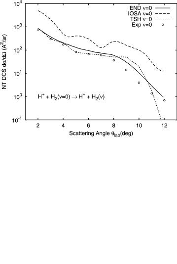
By using this approach, it is possible to calculate vibrational state-selected cross-sections from minimal END trajectories obtained with a classical description of the nuclei. We have studied vibrationally excited H2ðnÞ molecules produced in collisions with 30-eV protons [42,43]. The relevant experiments were performed by Toennies et al. [46] with comparisons to theoretical studies using the trajectory surface hopping model [11,47] (TSHM). This system has also stimulated a quantum mechanical study [48] using diatomics- in-molecule (DIM) surfaces [49] and invoking the infinite-order sudden approximation (IOSA).

In Figure 2, we show the total differential cross-section for product molecules in the vibrational ground state (no charge transfer) of the hydrogen molecule in collision with 30-eV protons in the laboratory frame. The experimental results that are in arbitrary units have been normalized to the END

Figure 2. Total differential cross-section versus laboratory scattering angle for vibrational ground state of hydrogen molecules in single collisioins with 30-eV protons.

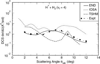
Figure 3. State resolved differential cross-section versus laboratory scattering angle for vibrational excitation of hydrogen molecules into state n ¼ 4 in single collisions with 30-eV protons.

results at the rainbow angle. The experimental estimate of the rainbow angle and the END calculated one are very close, 7 . The theoretical results using THSM and IOSA are shown for comparison. In Figure 3, the vibrational state resolved differential cross-section is shown for the fourth excited state (n ¼ 4). Results of similar quality are obtained for products in other vibrational states as long as the use of the harmonic oscillator coherent state can be justified.

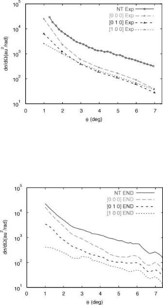
State resolved differential cross-sections for H2O in collisions with 46-eV protons in the center of mass were deduced [50] from time-of-flight energy loss spectra. The vibrational states are labeled ½n1; n2; n3&, where n1 denotes the number of quanta in the symmetric stretch mode, and n2 and n3, similarly denote the bending and asymmetric stretch, respectively. The experimental analysis assumes that the progressions ½n1; 0; 0& and ½n1; 1; 0& are the principal final states of the water molecules. This assumption is corroborated by our calculations. We show in Figure 4 the total differential cross-section for vibrational excitation (NT) and the state-resolved differential cross-sections for [0; 0; 0], [0; 1; 0], and [1; 0; 0]. The experimental energy resolution is such that it is not possible to distinguish between the symmetric and asymmetric stretching modes, so only one stretching mode is considered and denoted by n1.

The generalized Prony analysis of END trajectories for this system yield total and state resolved differential cross-sections. In Figure 5, we show the results. The theoretical analysis, which has no problem distinguishing between the symmetric and asymmetric stretch, shows that the asymmetric mode is only excited to a minor extent. The corresponding state resolved cross-section is about two orders of magnitude less than that of the symmetric stretch.

One reason that the symmetric stretch is favored over the asymmetric one might be the overall process, which is electron transfer. This means that most of the END trajectories show a nonvanishing probability for electron transfer and as a result the dominant forces try to open the bond angle during the collision toward a linear structure of H2Oþ. In this way, the totally symmetric bending mode is dynamically promoted, which couples to the symmetric stretch, but not to the asymmetric one.

Also, rotational state resolution of cross-sections can be obtained by employing a coherent state analysis [51] for the situation of weak coupling between rotational and vibrational degrees of freedom. A suitable rotational coherent state can be expressed as

IMK

where DIMK ða; b; gÞ ¼ e iaMdMKI e igK are rotational matrices [52], and where the angle parameters are related to the average values of the body fixed L and spacefixed J angular momentum components calculated with this coherent state, that is,

From these relations it follows that z is related to the angular momentum modulus, and that the pairs of angle a; b and g; d are the azimuthal, and the polar angle of the hJ2i and the hL2i vector, respectively. The angle E is associated with the relative orientation of the body-fixed and space-fixed coordinate frames. The probability to find the particular rotational state jIMKi in the coherent state is

The use of the rotational coherent state is then analogous to the use of the vibrational coherent state and can be used to study rotational state resolved properties. We note that the resolution of the identity applies here as well, that is,

X1 XI XI

I ¼ 0 M ¼ I K ¼ I

Final state analysis is where dynamical methods of evolving states meet the concepts of stationary states. By their definition, final states are relatively long lived. Therefore experiment often selects a single stationary state or a statistical mixture of stationary states. Since END evolution includes the possibility of electronic excitations, we analyze reaction products in terms of rovibronic states.

C.Intramolecular Electron Transfer

Minimal END has also been applied to a model system for intramolecular electron transfer. The small triatomic system LiHLi is bent C2v structure. But the linear structure presents an unrestricted Hartree–Fock (UHF) broken symmetry solution with the two charge localized structures

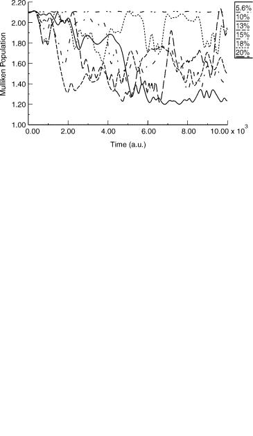
These charge-transfer structures have been studied [4] in terms a very limited number of END trajectories to model vibrational induced electron transfer. An electronic 3-21Gþ basis for Li [53] and 3-21G for H [54] was used. The equilibrium structure has the geometry with a long Li(2) H bond (3.45561 a.u.) and a short Li(1) H bond (3.09017 a.u.). It was first established that only the Li H bond stretching modes will promote electron transfer, and then initial conditions were chosen such that the long bond was stretched and the short bond compressed by the same (%) amount. The small ensemble of six trajectories with 5.6, 10, 13, 15, 18, and 20% initial change in equilibrium bond lengths are sufficient to illustrate the approach.

The END approach to electron-transfer processes is quite different from the current paradigm of Marcus theory, which due to its conceptual simplicity has guided much theoretical and experimental development. Introduced in the late 1950s [55], this theory has been extensively reviewed, revised, and extended [56–59]. This approach is characterized by the assumptions that there is a reaction coordinate that the reactants travel to the products and that there is a coupling H12 between the donor and acceptor states. Figure 6 shows a typical picture of participating adiabatic and diabatic states along a reaction coordinate for normal electron transfer according to the Marcus theory. END by its very nature constructs dynamical trajectories in wave function phase space, including the electronic degrees of freedom, from which transition probabilities are obtained. In this approach, there is no need to break the transfer process into two separate steps, that is geometry change and electronic transition. Instead END describes the full evolution and the coupling of these two aspects of the process. Initiation of electron transfer is accomplished by simply distorting the molecule and letting the system evolve in time.

A simple measure of the electron density distribution over the participating atoms is the Mulliken population [60]. For linear Li H Li the alpha spin is

Figure 6. Diabatic and corresponding adiabatic potential energy along a relevant reaction coordinate for normal electron transfer.

arbitrarily chosen in excess in the single determinantal electronic state. In Figure 7, the alpha Mulliken populations are shown for the six END trajectories over 10,000 a.u. of time.

A transfer rate constant can be obtained by applying a Boltzmann distribution, and by writing the concentration of reactant present as

X

XðtÞ ¼ eEn=kT PnðtÞ ð68Þ

n

Figure 7. Alpha Mulliken population on Li(2) as functions of time for different initial conditions.

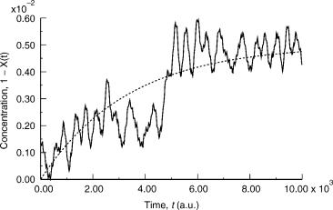
Figure 8. Concentration of the product species as a function of time.

where En is the energy above the ground state and Pn the probability of electron transfer for initial state n. The electron transfer in this case is effectively a oneelectron process and since for such a case the transfer probability is directly related to the Mulliken population one may write

where Mn is the alpha Mulliken population on Li(2) for initial state n, and Mnmax is the maximum value of this population. In this case, MNmax ¼ 2 and Pn becomes a number between 0 and 1 yielding the probability that an electron will move from Li(2) to Li(1).

The small statistical sample leaves strong fluctuations on the timescale of the nuclear vibrations, which is a behavior typical of any detailed microscopic dynamics used as data for a statistical treatment to obtain macroscopic quantities.

However, as can be seen from Figure 8 a simple exponential expected from first-order kinetics can be fitted to the data yielding a limiting concentration of 0.005, and a rate constant of 0.0003 a.u., which translates to 1:25 1013 s 1 at 300 K.

References

¨

1. Y. Ohrn et al., in Time-Dependent Quantum Molecular Dynamics, J. Broeckhove and L. Lathouwers, eds., Plenum, New York, 1992, pp. 279–292.

¨

2. E. Deumens, A. Diz, H. Taylor, and Y. Ohrn, J. Chem. Phys. 96, 6820 (1992).