Baer M., Billing G.D. (eds.) - The role of degenerate states in chemistry (Adv.Chem.Phys. special issue, Wiley, 2002)

applying direct molecular dynamics to non-adiabatic systems 363

In what is called BO MD, the nuclear wavepacket is simulated by a swarm of trajectories. We emphasize here that this does not necessarily mean that the nuclei are being treated classically. The difference is in the chosen initial conditions. A fully classical treatment takes the initial positions and momenta from a classical ensemble. The use of quantum mechanical distributions instead leads to a semiclassical simulation. The important topic of choosing initial conditions is the subject of Section II.C.

Finally, Gaussian wavepacket methods are described in which the nuclear wavepacket is described by one or more Gaussian functions. Again the equations of motion to be solved have the form of classical trajectories in phase space. Now, however, each trajectory has a quantum character due to its spread in coordinate space.

A.Quantum Wavepacket Propagation

Using the BO approximation, the Schro¨dinger equation describing the time evolution of the nuclear wave function, wðR; tÞ, can be written

In this picture, the nuclei are moving over a PES provided by the function VðRÞ,

^

driven by the nuclear kinetic energy operator, TN . More details on the derivation of this equation and its validity are given in Appendix A. The potential function is provided by the solutions to the electronic Schro¨dinger equation,

where Hel is the electronic (clamped nucleus) Hamiltonian defined in Eq. (6). In this equation it must be remembered that R is a parameter defining the nuclear configuration, and cðr; RÞ an electronic eigenfunction at this configuration. A PES is thus formed by following one of the roots of this equation (e.g., the second root for the first excited state) as the nuclear geometry changes. Approximate solutions to this equation are the results of the standard quantum chemistry computer packages, such as GAUSSIAN [95], GAMESS [96], MOLCAS [97], MOLPRO [98], and COLUMBUS [99].

To solve this equation, an appropriate basis set ffaðRÞg is required for the nuclear functions. These could be a set of harmonic oscillator functions if the motion to be described takes place in a potential well. For general problems, a discrete variable representation (DVR) [100,101] is more suited. These functions have mathematical properties that allow both the kinetic and potential energy

operators to be easily represented. In coordinate space, they are effectively d functions, and so the potential can be represented on a grid of points. The wave function is then expanded in this set

where the nuclear function is a vector in the space provided by the basis, that is, the components are the expansion coefficients ca, and the Hamiltonian matrix elements are

If VðRÞ is known and the matrix elements Hab are evaluated, then solution of Eq. (10) for a given initial wavepacket is the numerically exact solution to the Schro¨dinger equation.

Efficient techniques for the direct solution of Eq. (10) have been developed using either a DVR or FFT-based method [102] to generate a representation of the wavepacket and Hamiltonian on a grid in coordinate space [15,16,18,103]. In principle, the differential equation can be directly solved, using a standard integrator (predictor–corrector, Runge–Kutte, etc.) to propagate the vector v forward in time using the time derivative, which is calculated using simple matrix–vector multiplication. Alternatively, for a time-independent Hamiltonian, Eq. (10) can be written in integral form

The problem is then reduced to the representation of the time-evolution operator [104,105]. For example, the Lanczos algorithm could be used to generate the eigenvalues of H, which can be used to set up the representation of the exponentiated operator. Again, the methods are based on matrix–vector operations, but now much larger steps are possible.

Unfortunately, the resources required for these numerically exact methods grow exponentially with the number of degrees of freedom in the system of interest. Without the use of clever algorithms to optimize the basis set used [106,107], this limits the range of systems treatable to 4–6 degrees of freedom (3–4 atoms). For larger systems, the MCTDH method [19,20,108] provides a

applying direct molecular dynamics to non-adiabatic systems 365

flexible, yet accurate method. This method uses a time-dependent basis set, and has treated, for example, the dynamics of the pyrazine molecule after photoexcitation including all 24 vibrational modes and 2 coupled electronic states [109]. A time-dependent basis is efficient because it follows the evolving wavepacket, and does not waste effort in describing regions of empty space. In effect, the semiclassical methods described below are using a set of classical trajectories or Gaussian wavepackets as a time-dependent basis set. The connection between the MCTDH basis functions and trajectories has recently been explored [110], and it has been shown that a set of coupled trajectories can act as a basis set for full quantum dynamics calculations. The connection between a time-dependent basis set and the Gaussian wavepacket methods is more obvious.

Before progressing, it is useful to review the dynamics of typical molecular systems. We consider three types: scattering (chemical reaction), photodissociation, and bound-state photoabsorption (no reaction).

The H þ H2 ! H2 þ H hydrogen atom exchange reaction is the simplest atom–molecule scattering system. Molecules and atoms colliding is a basic step in chemical reactivity, and much work has been made to understand this system in all its details [111,112]. As well as experimental work, extensive calculations have been made using both a time-independent framework [113] and wavepacket methods [114–116] to obtain fully state resolved cross-sections for the reaction. This system is best described by Jacobi coordinates, shown in Figure 1a, and the reaction is dominated by the colinear configuration. The PES for this configuration (i.e., a cut with y ¼ 0 ) has a C-shaped minimum energy channel, with a saddle point as a transition region at the apex. This is shown in Figure 2.

The evolution of a wavepacket representing the H þ H2 scattering reaction for a particular set of initial conditions is plotted on Figure 2 as a series of snapshots. To display the three-dimensional (3D) wavepacket on a two-dimensional (2D) plot, the reduced density

is plotted. The system stays close to the colinear configuration, and so integrating over the angular coordinate does not lead to significant loss of information. Note, however, that the results from a 2D calculation in which the angle is kept fixed would be different.

In the reactant channel leading up to the transition region, motion along Rd represents the H atom approaching the molecule, while motion along Rv is the vibrational motion of the atom. The initial wavepacket is chosen to represent the desired initial conditions. In Figure 2, the H2 molecule is initially in the ground

Figure 1. Coordinates used for describing the dynamics of (a) H þ H2 (b) NOCl, (c) butatriene. (a), (b) Are Jacobi coordinates, where Rd and Rv are the dissociative and vibrational coordinates, respectively. (c) Shows the two most important normal mode coordinates, Q5 and Q14 which are the torsional and central C C bond stretch, respectively.

vibrational state, and the atom is located relative to the molecule by a Gaussian distribution of positions, moving with an initial momentum toward the molecule. The initial packet is thus close to a product of Gaussian functions. The quantum mechanical nature of the system means that the wavepacket possesses a distribution of momenta, and therefore energies. The figure shows how the wavepacket moves along the reactant channel, and is split as it hits the energy barrier representing the molecule–atom collision. Part of the packet moves on into the product channel (hydrogen atom exchange), and part is reflected back to the reactants (no exchange). The wavepacket can then be analyzed to obtain information about the transfer of population from the initial state to the final states over the energies contained in the packet.

A different category of dynamics is found in photodissociation processes, in which a molecule breaks up after absorbing a photon. A simple example is found in the NOCl molecule after excitation to the first singlet, S1, state [117]. The molecule is initially in the ground vibrational state on the ground electronic surface. After the photoexcitation, this nuclear wave function is moved vertically onto the excited state. The S1 PES as calculated by Schinke et al. [118] is shown in Figure 3. This is again in Jacobi coordinates, which are shown in Figure 1b. For the plot the angular coordinate, which plays only a minor role in the process, is at the ground-state equilibrium value of 127 .

The evolution of the nuclear wavepacket is also traced by a number of snapshots of the absolute values of the wavepacket, again integrating over the

Figure 3. Wavepacket dynamics of the photodissociation of NOCl, shown as snapshots of the density (wavepacket amplitude squared) at various times. The coordinates, in au, are described in Figure 1b, and the wavepacket is initially the ground-state vibronic wave function vertically excited onto the S1 state. Increasing Rd corresponds to chlorine dissociation. The density has been integrated over the angular coordinate. The S1 PES is ploted for the geometry, y ¼ 127 , the ground-state equilibrium value.

angular coordinate. The wavepacket evolves away from its initial Gaussian-like form down the valley, which leads to direct dissociation. The structure formed in the wavepacket leads to structure in the absorption spectrum, which is absent if the angle y is frozen, and is thus due to the flow of energy between the bend and stretch motions. Even more complicated behavior would be found if the PES contained a barrier to the dissociation, which would lead to a break up of the packet.

applying direct molecular dynamics to non-adiabatic systems 369

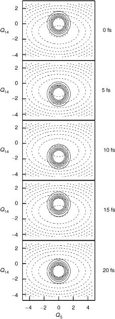
The third major category of processes are dynamics after bound–bound transitions, such as photoexcitation to a bound state. In Figure 4, the system dynamics of the butatriene radical cation are shown after excitation from the neutral molecule ground state to a simple model of the cationic first excited state, a process related to the first excited band in the photoelectron spectrum. The dynamics are dominated by two vibrational modes, the central C C stretch, labeled Q14 and the torsion, Q5. These coordinates are shown in Figure 1c. In this simple model, the PES is taken as a harmonic approximation around the minimum energy point, which is found to be shifted along the Q14 mode. Here, non-adiabatic effects have been ignored. As will be shown in Section III.D, there is in fact strong vibronic coupling to the cationic ground state via the torsional mode, and the true dynamics after excitation into this state is radically altered. This model is, however, a reasonable representation of a bound state in which vibronic coupling does not play a role. The systems dynamics in the space of the two normal modes shown is fairly simple. The initial Gaussian shaped wavepacket representing the neutral ground-state wave function moves back and forth across the well, driven by the initial force due to the shifted energy minimum.

For bound state systems, eigenfunctions of the nuclear Hamiltonian can be found by diagonalization of the Hamiltonian matrix in Eq. (11). These functions are the possible nuclear states of the system, that is, the vibrational states. If these states are used as a basis set, the wave function after excitation is a superposition of these vibrational states, with expansion coefficients given by the Frank–Condon overlaps. In this picture, the dynamics in Figure 4 can be described by the time evolution of these expansion coefficients, a simple phase factor. The periodic motion in coordinate space is thus related to a discrete spectrum in energy space.

B.Born–Oppenheimer Molecular Dynamics

In a classical limit of the Schro¨dinger equation, the evolution of the nuclear wave function can be rewritten as an ensemble of pseudoparticles evolving under Newton’s equations of motion

where VðRÞ is the potential and is the second-derivative with respect to time of

R

the position, that is, the acceleration. They are referred to as pseudoparticle trajectories as, as explained above, the ensemble might be simulating the motion of a quantum wavepacket, in which case a single particle is being represented by a number of pseudoparticles.

This picture is often referred to as ‘‘swarms of trajectories,’’ and details are given in Appendix B. The nuclear problem is thus reduced to solving Newton’s equations of motion for a number of different starting conditions. To connect

applying direct molecular dynamics to non-adiabatic systems 371

this picture to the delocalized quantum mechanical one, the wavepacket is being represented by a time-dependent basis set of ‘‘functions’’ that are the points describing the trajectory of the classical pseudoparticle. The nuclear wavepacket is then being approximated by a vector, the elements of which are the populations of the trajectories in the initial ensemble.

The force experienced by a pseudoparticle is simply

where ra is a component of the derivative operator in coordinate space. The obvious approach is thus to calculate the electronic wave function at time t, and then directly calculate the required derivatives. The nuclei can then be propagated forward a step, and the process repeated. This algorithm is usually termed BO dynamics, and it was the method used in the first direct dynamics studies [66–68].

While it is conceptually simple, however, the method suffers from the expense of requiring the full electronic wave function at each step, for example, by solving the electronic structure problem using an SCF technique. For the method to be feasible, a large time-step is therefore required to minimise the number of these expensive evaluations that need to be made. Classical MD simulations typically use integration schemes based on either the Gear predictor-corrector [119] or the Verlet [120] algorithms (see [121] for overview of these methods, and [122] for other useful integrators). These give reasonable time-steps with low memory requirements for large systems, and require only first derivatives of the potential, the forces, at each step.

A different approach comes from the idea, first suggested by Helgaker et al. [77], of approximating the PES at each point by a harmonic model. Integration within an area where this model is appropriate, termed the trust radius, is then trivial. Normal coordinates, Q, are defined by diagonalization of the massweighted Hessian (second-derivative) matrix, so if

where R0 is the present position, then

where x2 is the (diagonal) matrix of eigenvalues from transforming the massweighted Hessian, H, using the unitary matrix L, and g and G are the forces (first

derivatives) in the two coordinate sets. The diagonal matrix m contains the masses associated with each coordinates. If R0 is a minimum on the PES, then x are the vibrational frequencies, and Q the vibrational modes of the molecule.

In this representation, Newton’s equations of motion separate to 3N 6 equations

that have different analytical solutions depending on whether the ‘‘frequency’’ o is real, zero, or imaginary. These solutions are used to integrate the equations of motion from R0 to Rt, where t is controlled by the trust radius. This radius changes, guided by the difference between the information about the PES calculated at xt, and that estimated from the harmonic model.

This algorithm was improved by Chen et al. [78] to take into account the surface anharmonicity. After taking a step from R0 to R0t using the harmonic approximation, the true surface information at R0t is then used to fit a (fifthorder) polynomial to form a better model of the surface. This polynomial model is then used in a corrector step to give the new Rt.

The Helgaker–Chen algorithm results in very large steps being possible, and despite the extra cost of the required second derivatives, this is the method of choice for direct dynamics calculations. A number of systems have been treated, and a review of the method as applied to chemical reactions is given in [2].

The gradient of the PES (force) can in principle be calculated by finite difference methods. This is, however, extremely inefficient, requiring many evaluations of the wave function. Gradient methods in quantum chemistry are fortunately now very advanced, and analytic gradients are available for a wide variety of ab initio methods [123–127]. Note that if the wave function depends on a set of parameters {l}, for example, the expansion coefficients of the basis functions used to build the orbitals in molecular orbital (MO) theory,

where V is defined in Eqs. (15) and (16). If the wave function is derived using a variational method, then qV=qli ¼ 0. Further, if the basis set is independent of R, which is the case when it is complete, then Eq. (23) can be used to show that