

Biomechanics Principles and Applications - Donald R. Peterson & Joseph D. Bronzino
.pdf3-2 |
|
Biomechanics |
Sliding |
Spinning |
Rolling |
ICR
S1
|
ICR |
ICR at |
S1 = S2 |
S2
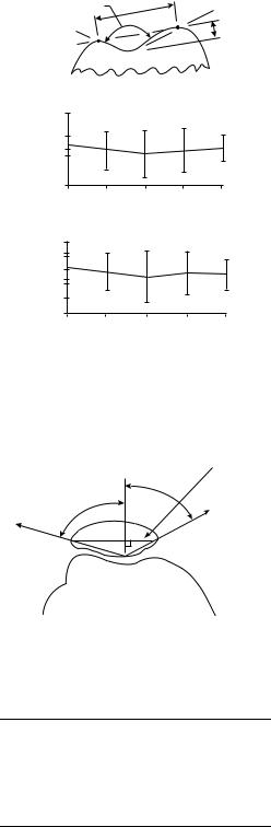
FIGURE 3.1 Three types of articulating surface motion in human joints.
Various degrees of simplification have been used for kinematic modeling of joints. A hinged joint is the simplest and most common model used to simulate an anatomic joint in planar motion about a single axis embedded in the fixed segment. Experimental methods have been developed for determination of the instantaneous center of rotation for planar motion. The instantaneous center of rotation is defined as the point of zero velocity. For a true hinged motion, the instantaneous center of rotation will be a fixed point throughout the movement. Otherwise, loci of the instantaneous center of rotation or centrodes will exist. The center of curvature has also been used to define joint anatomy. The center of curvature is defined as the geometric center of coordinates of the articulating surface.
For more general planar motion of an articulating surface, the term sliding, rolling, and spinning are commonly used (Figure 3.1). Sliding (gliding) motion is defined as the pure translation of a moving segment against the surface of a fixed segment. The contact point of the moving segment does not change, while the contact point of the fixed segment has a constantly changing contact point. If the surface of the fixed segment is flat, the instantaneous center of rotation is located at infinity. Otherwise, it is located at the center of curvature of the fixed surface. Spinning motion (rotation) is the exact opposite of sliding motion. In this case, the moving segment rotates, and the contact points on the fixed surface does not change. The instantaneous center of rotation is located at the center of curvature of the spinning body that is undergoing pure rotation. Rolling motion occurs between moving and fixed segments where the contact points in each surface are constantly changing and the arc lengths of contact are equal on each segment. The instantaneous center of rolling motion is located at the contact point. Most planar motion of anatomic joints can be described by using any two of these three basic descriptions.
In this chapter, various aspects of joint-articulating motion are covered. Topics include the anatomical characteristics, joint contact, and axes of rotation. Joints of both the upper and lower extremity are discussed.
3.1 Ankle
The ankle joint is composed of two joints: the talocrural (ankle) joint and the talocalcaneal (subtalar joint). The talocrural joint is formed by the articulation of the distal tibia and fibula with the trochlea of the talus. The talocalcaneal joint is formed by the articulation of the talus with the calcaneus.
3.1.1 Geometry of the Articulating Surfaces
The upper articular surface of the talus is wedge-shaped, its width diminishing from front to back. The talus can be represented by a conical surface. The wedge shape of the talus is about 25% wider in front than behind with an average difference of 2.4 ± 1.3 mm and a maximal difference of 6 mm [Inman, 1976].
3.1.2 Joint Contact
The talocrural joint contact area varies with flexion of the ankle (Table 3.1). During plantarflexion, such as would occur during the early stance phase of gait, the contact area is limited and the joint is incongruous.
Joint-Articulating Surface Motion |
|
|
3-3 |
||
|
TABLE 3.1 Talocalcaneal (Ankle) Joint Contact Area |
|
|
||
|
|
|
|
|
|
|
Investigators |
Plantarflexion |
Neutral |
Dorsiflexion |
|
|
|
|
|
|
|
|
Ramsey and Hamilton [1976] |
|
4.40 ± 1.21 |
|
|
|
Kimizuki et al. [1980] |
|
4.83 |
|
|
|
Libotte et al. [1982] |
5.01 (30◦ ) |
5.41 |
3.60 (30◦ ) |
|
|
Paar et al. [1983] |
4.15 (10◦ ) |
4.15 |
3.63 (10◦ ) |
|
|
Macko et al. [1991] |
3.81 ± 0.93 (15◦ ) |
5.2 ± 0.94 |
5.40 ± 0.74 (10◦ ) |
|
|
Driscoll et al. [1994] |
2.70 ± 0.41 (20◦ ) |
3.27 ± 0.32 |
2.84 ± 0.43 (20◦ ) |
|
|
Hartford et al. [1995] |
1.49 (20◦ ) |
3.37 ± 0.52 |
1.47 (10◦ ) |
|
|
Pereira et al. [1996] |
1.67 |
|||
|
Rosenbaum et al. [2003] |
|
2.11 ± 0.72 |
|
|
Note: The contact area is expressed in square centimeters.
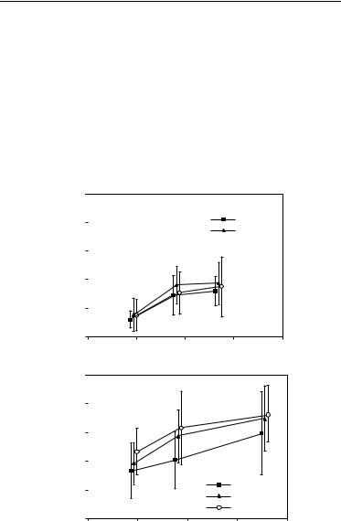
As the position of the joint progresses from neutral to dorsiflexion, as would occur during the midstance of gait, the contact area increases and the joint becomes more stable. The area of the subtalar articulation is smaller than that of the talocrural joint. The contact area of the subtalar joint is 0.89 ± 0.21 cm2 for the posterior facet and 0.28 ± 15 cm2 for the anterior and middle facets [Wang et al., 1994]. The total contact area (1.18 ± 0.35 cm2) is only 12.7% of the whole subtalar articulation area (9.31 ± 0.66 cm2) [Wang et al., 1994]. The contact area/joint area ratio increases with increases in applied load (Figure 3.2).
(a) |
|
0.5 |
|
|
|
||
contactofRatioarea |
areajointto |
0.4 |
|
0.3 |
|
||
|
|
|
|
|
|
0.2 |
|
|
|
0.1 |
|
|
|
0.0 |
|
|
|
|
|
|
|
0 |
|
(b) |
|
1.0 |
|
|
|
||
|
|
|
|
contactofRatioarea |
areajointto |
0.8 |
|
0.6 |
|
||
|
|
|
|
|
|
0.4 |
|
|
|
0.2 |
|
|
|
0.0 |
|
|
|
|
|
|
|
0 |
|
Inverted
Neutral
 Everted
400 |
800 |
1200 |
1600 |
|
Axial load (N) |
|
|
|
|
Inverted |
|
|
|
Neutral |
|
|
|
Everted |
|
400 |
800 |
1200 |
1600 |
Axial load (N)
FIGURE 3.2 Ratio of total contact area to joint area in the (a) anterior/middle facet and (b) posterior facet of the subtalar joint as a function of applied axial load for three different positions of the foot. (From Wagner U.A., Sangeorzan B.J., Harrington R.M., and Tencer A.F. 1992. J. Orthop. Res. 10: 535. With permission.)

3-4 |
|
Biomechanics |
||
|
TABLE 3.2 Axis of Rotation for the Ankle |
|||
|
|
|
|
|
|
Investigators |
Axisa |
Position |
|
|
Elftman [1945] |
Fix. |
67.6 ± 7.4◦ with respect to sagittal plane |
|
|
Isman and Inman [1969] |
Fix. |
8 mm anterior, 3 mm inferior to the distal tip of the lateral malleolus; 1 mm posterior, |
|
|
|
|
5 mm inferior to the distal tip of the medial malleolus |
|
|
Inman and Mann [1979] |
Fix. |
79◦ (68–88◦ ) with respect to the sagittal plane |
|
|
Allard et al. [1987] |
Fix. |
95.4 ± 6.6◦ with respect to the frontal plane, 77.7 ± 12.3◦ with respect to the sagittal |
|
|
|
|
plane, and 17.9 ± 4.5◦ with respect to the transverse plane |
|
|
Singh et al. [1992] |
Fix. |
3.0 mm anterior, 2.5 mm inferior to distal tip of lateral malleolus; 2.2 mm posterior, |
|
|
|
|
10 mm inferior to distal tip of medial malleolus |
|
|
Sammarco et al. [1973] |
Ins. |
Inside and outside the body of the talus |
|
|
D’Ambrosia et al. [1976] |
Ins. |
No consistent pattern |
|
|
Parlasca et al. [1979] |
Ins. |
96% within 12 mm of a point 20 mm below the articular surface of the tibia along |
|
|
|
|
the long axis |
|
|
Van Langelaan [1983] |
Ins. |
At an approximate right angle to the longitudinal direction of the foot, passing |
|
|
|
|
through the corpus tali, with a direction from anterolaterosuperior to posterome- |
|
|
|
|
dioinferior |
|
|
Barnett and Napier |
Q-I |
Dorsiflexion: down and lateral |
|
|
|
|
Plantarflexion: down and medial |
|
|
Hicks [1953] |
Q-I |
Dorsiflexion: 5 mm inferior to tip of lateral malleolus to 15 mm anterior to tip of |
|
|
|
|
medial malleolus |
|
|
|
|
Plantarflexion: 5 mm superior to tip of lateral malleolus to 15 mm anterior, 10 mm |
|
|
|
|
inferior to tip of medial malleolus |
|
a Fix. = fixed axis of rotation; Ins. = instantaneous axis of rotation; Q-I = quasi-instantaneous axis of rotation.
3.1.3 Axes of Rotation
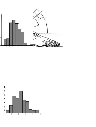
Joint motion of the talocrural joint has been studied to define the axes of rotation and their location with respect to specific anatomic landmarks (Table 3.2). The axis of motion of the talocrural joint essentially passes through the inferior tibia at the fibular and tibial malleoli (Figure 3.3). Three types of motion have been used to describe the axes of rotation: fixed, quasi-instantaneous, and instantaneous axes. The motion
|
|
|
Obliquity of ankle axis |
||
Number |
|
|
|
|
|
of |
|
|
|
|
|
specimens |
|
|
|
|
|
20 |
|
|
|
|
– |
|
|
|
|
x=82° |
|
15 |
|
|
|
|
|
|
|
|
|
|
74° |
10 |
|
|
|
|
94° |
|
|
|
|
|
|
5 |
|
|
|
|
|
74 |
78 |
82 |
86 |
96 |
94 |
|
|
Angle (degrees) |
|
|
|
|
– |
|
.6 |
.=x+3 |
|||
S.D |
|
– |
|
FIGURE 3.3 Variations in angle between middle of tibia and empirical axis of ankle. The histogram reveals a considerable spread of individual values. (From Inman V.T. 1976. The Joints of the Ankle, Baltimore, Williams and Wilkins. With permission.)

Joint-Articulating Surface Motion |
3-5 |
||||
|
TABLE 3.3 Axis of Rotation for the Talocalcaneal (Subtalar) Joint |
|
|
||
|
|
|
|
|
|
|
Investigators |
Axisa |
Position |
|
|
|
Manter [1941] |
Fix. |
16◦ (8–24◦ ) with respect to sagittal plane, and 42◦ (29–47◦ ) with respect to transverse |
||
|
|
|
plane |
|
|
|
Shephard [1951] |
Fix. |
Tuberosity of the calcaneus to the neck of the talus |
|
|
|
Hicks [1953] |
Fix. |
Posterolateral corner of the heel to superomedial aspect of the neck of the talus |
|
|
|
Root et al. [1966] |
Fix. |
17◦ (8–29◦ ) with respect to sagittal plane, and 41◦ (22–55◦ ) with respect to transverse |
||
|
|
|
plane |
|
|
|
Isman and Inman [1969] |
Fix. |
23◦ ± 11◦ with respect to sagittal plane, and 41◦ ± 9◦ with respect to transverse plane |
||
|
Kirby [1947] |
Fix. |
Extends from the posterolateral heel, posteriorly, to the first intermetatarsal space, |
||
|
|
|
anteriorly |
|
|
|
Rastegar et al. [1980] |
Ins. |
Instant centers of rotation pathways in posterolateral quadrant of the distal articu- |
||
|
|
|
lating tibial surface, varying with applied load |
|
|
|
Van Langelaan [1983] |
Ins. |
A bundle of axes that make an acute angle with the longitudinal direction of the |
||
|
|
|
foot passing through the tarsal canal having a direction from anteromediosuperior |
||
|
|
|
to posterolateroinferior |
|
|
|
Engsberg [1987] |
Ins. |
A bundle of axes with a direction from anteromediosuperior to posterolateroinferior |
||
a Fix. = fixed axis of rotation; Ins. = instantaneous axis of rotation.
that occurs in the ankle joints consists of dorsiflexion and plantarflexion. Minimal or no transverse rotation takes place within the talocrural joint. The motion in the talocrural joint is intimately related to the motion in the talocalcaneal joint, which is described next.
The motion axes of the talocalcaneal joint have been described by several authors (Table 3.3). The axis of motion in the talocalcaneal joint passes from the anterior medial superior aspect of the navicular bone to the posterior lateral inferior aspect of the calcaneus (Figure 3.4). The motion that occurs in the talocalcaneal joint consists of inversion and eversion.
3.2 Knee
The knee is the intermediate joint of the lower limb. It is composed of the distal femur and proximal tibia. It is the largest and most complex joint in the body. The knee joint is composed of the tibiofemoral articulation and the patellofemoral articulation.
3.2.1 Geometry of the Articulating Surfaces
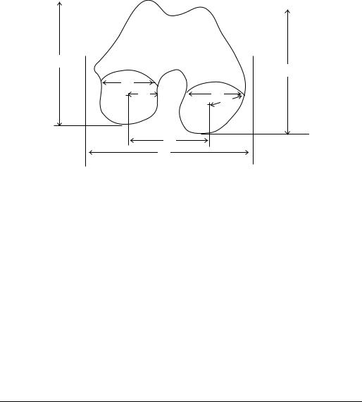
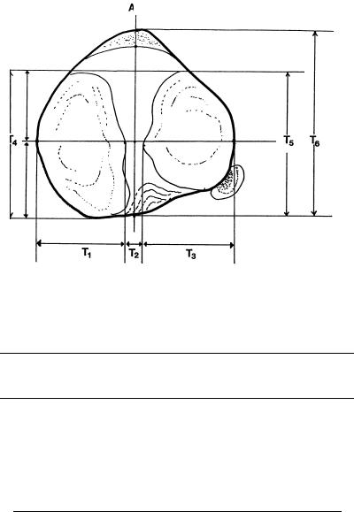
The shape of the articular surfaces of the proximal tibia and distal femur must fulfill the requirement that they move in contact with one another. The profile of the femoral condyles varies with the condyle examined (Figure 3.5 and Table 3.4). The tibial plateau widths are greater than the corresponding widths of the femoral condyles (Figure 3.6 and Table 3.6). However, the tibial plateau depths are less than those of the femoral condyle distances. The medial condyle of the tibia is concave superiorly (the center of curvature lies above the tibial surface) with a radius of curvature of 80 mm [Kapandji, 1987]. The lateral condyle is convex superiorly (the center of curvature lies below the tibial surface) with a radius of curvature of 70 mm [Kapandji, 1987]. The shape of the femoral surfaces is complementary to the shape of the tibial plateaus. The shape of the posterior femoral condyles may be approximated by spherical surfaces (Table 3.4).
The geometry of the patellofemoral articular surfaces remains relatively constant as the knee flexes. The knee sulcus angle changes only ±3.4◦ from 15 to 75◦ of knee flexion (Figure 3.7). The mean depth index varies by only ±4% over the same flexion range (Figure 3.7). Similarly, the medial and lateral patellar facet angles (Figure 3.8) change by less than a degree throughout the entire knee flexion range (Table 3.7). However, there is a significant difference between the magnitude of the medial and lateral patellar facet angles.
3-6 |
Biomechanics |
(a) Number of
specimens 20
15 |
|
|
|
|
|
10 |
|
|
|
|
|
5 |
|
|
|
|
|
20 |
30 |
40 |
50 |
60 |
70 |
|
Angle (degrees) |
|
|||
(b)
Number |
|
|
Midline |
of |
|
– |
° |
specimens |
S.D.= 11° |
x=23 |
|
|
4° |
||
20 |
|
|
|
15 |
|
|
|
47° |
Range |
|
|
|
|
|
|
10 |
|
|
|
|
|
5 |
|
|
|
|
|
0 |
10 |
20 |
30 |
40 |
50 |
|
Angle (degrees) |
|
|||
|
|
of |
– |
talocalcaneal |
|
S.D.=x+9 |
Axis |
|
– |
|
joint |
68.5° |
|
|
|
|
|
Range
– ° x=42
20.5°
Horiz. plane
FIGURE 3.4 (a) Variations in inclination of axis of subtalar joint as projected upon the sagittal plane. The distribution of the measurements on the individual specimens is shown in the histogram. The single observation of an angle of almost 70◦ was present in a markedly cavus foot. (b) Variations in position of subtalar axis as projected onto the transverse plane. The angle was measured between the axis and the midline of the foot. The extent of individual variation is shown on the sketch and revealed in the histogram. (From Inman V.T. 1976. The Joints of the Ankle, Baltimore, Williams and Wilkins. With permission.)
3.2.2 Joint Contact
The mechanism for movement between the femur and tibia is a combination of rolling and gliding. Backward movement of the femur on the tibia during flexion has long been observed in the human knee. The magnitude of the rolling and gliding changes through the range of flexion. The tibial-femoral contact point has been shown to move posteriorly as the knee is flexed, reflecting the coupling of posterior motion with flexion (Figure 3.9). In the intact knee at full extension, the center of pressure is approximately 25 mm from the anterior edge of the tibial plateau [Andriacchi et al., 1986]. The medial femoral condyle rests further anteriorly on the tibial plateau than the lateral plateau. The medial femoral condyle is positioned 35 ± 4 mm from the posterior edge while the lateral femoral condyle is positioned 25 ± 4 mm from the posterior edge (Figure 3.9). During knee flexion to 90◦, the medial femoral condyle moves back 15 ± 2 mm
Joint-Articulating Surface Motion |
3-7 |
|||
|
|
|
|
|
|
|
|
|
|
K3
K4
K1
K6 |
K2 |
K7
|
K8 |
|
K5 |
Lateral |
Medial |
FIGURE 3.5 Geometry of distal femur. The distances are defined in Table 3.4.
and the lateral femoral condyle moves back 12 ± 2 mm. Thus, during flexion the femur moves posteriorly on the tibia (Table 3.9).
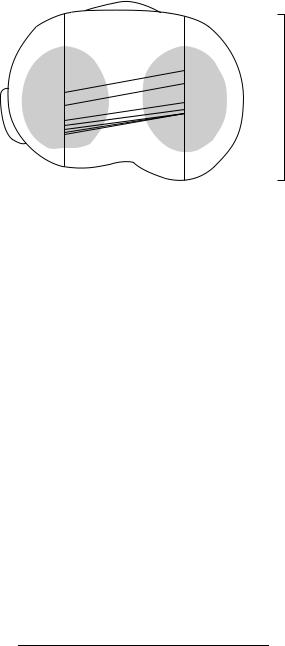
The patellofemoral contact area is smaller than the tibiofemoral contact area (Table 3.10). As the knee joint moves from extension to flexion, a band of contact moves upward over the patellar surface (Figure 3.10). As knee flexion increases, not only does the contact area move superiorly, but it also becomes larger. At 90◦ of knee flexion, the contact area has reached the upper level of the patella. As the knee continues to flex, the contact area is divided into separate medial and lateral zones.
3.2.3 Axes of Rotation
The tibiofemoral joint is mainly a joint with two degrees of freedom. The first degree of freedom allows movements of flexion and extension in the sagittal plane. The axis of rotation lies perpendicular to the sagittal plane and intersects the femoral condyles. Both fixed axes and screw axes have been calculated
TABLE 3.4 Geometry of the Distal Femur
|
|
|
|
|
Condyle |
|
|
|
|
|
|
|
|
|||
|
|
|
|
|
|
|
|
|
|
|
|
|
|
|
||
|
|
|
Lateral |
|
|
|
|
Medial |
|
|
|
|
|
Overall |
||
|
|
|
|
|
|
|
|
|
|
|
|
|||||
Parameter |
Symbol |
Distance (mm) |
Symbol |
Distance (mm) |
Symbol |
Distance (mm) |
||||||||||
|
|
|
|
|
|
|
|
|
|
|
|
|||||
Medial/lateral distance |
|
K1 |
31 |
± 2.3 (male) |
|
K2 |
32 |
± 31 (male) |
|
|
|
|||||
Anterior/posterior distance |
|
K3 |
28 |
± 1.8 |
(female) |
|
|
27 |
± 3.1 |
(female) |
|
|
|
|||
|
72 |
± 4.0 |
(male) |
|
K4 |
70 |
± 4.3 |
(male) |
|
|
|
|||||
Posterior femoral condyle |
|
K6 |
65 |
± 3.7 |
(female) |
|
|
63 |
± 4.5 |
(female) |
|
|
|
|||
|
19.2 ± 1.7 |
|
|
K7 |
20.8 ± 2.4 |
|
|
|
|
|
||||||
spherical radii |
|
|
|
|
|
|
|
|
|
|
|
|
|
|
|
90 ± 6 (male) |
Epicondylar width |
|
|
|
|
|
|
|
|
|
|
|
|
|
|
K5 |
|
|
|
|
|
|
|
|
|
|
|
|
|
|
|
|
|
80 ± 6 (female) |
Medial/lateral spacing of |
|
|
|
|
|
|
|
|
|
|
|
|
|
|
K8 |
45.9 ± 3.4 |
center of spherical surfaces |
|
|
|
|
|
|
|
|
|
|
|
|
|
|
|
|
|
|
|
|
|
|
|
|
|
|
|
|
|
|
|
|
|
Note: See Figure 3.5 for location of measurements.
Source: Yoshioka Y., Siu D., and Cooke T.D.V. 1987. J. Bone Joint Surg. 69A: 873–880. Kurosawa H., Walker P.S., Abe S., Garg A., and Hunter T. 1985. J. Biomech. 18: 487.
3-8 |
Biomechanics |
AP
T4 |
|
T5 |
|
T6 |
T1 |
|
T2 |
|
T3 |
|
|
|
|
|
FIGURE 3.6 Contour of the tibial plateau (transverse plane). The distances are defined in Table 3.6.
TABLE 3.5 Posterior Femoral Condyle Spherical Radius
|
Normal Knee |
Varus Knees |
Valgus Knees |
Medial condyle |
20.3 ± 3.4(16.1–28.0) |
21.2 ± 2.1(18.0–24.5) |
21.1 ± 2.0(17.84–24.1) |
Lateral condyle |
19.0 ± 3.0(14.7–25.0) |
20.8 ± 2.1(17.5–30.0) |
21.1 ± 2.1(18.4–25.5) |
Significantly different from normal knees ( p < 0.05).
Source: Matsuda S., Miura H., Nagamine R., Mawatari T., Tokunaga M., Nabeyama R., and
Iwamoto Y. Anatomical analysis of the femoral condyle in normal and osteoarthritic knees. J. Ortho. Res. 22: 104–109, 2004.
TABLE 3.6 Geometry of the Proximal Tibia
Parameter |
Symbols |
All limbs |
Male |
Female |
|
|
|
|
|
Tibial plateau with widths (mm) |
|
32 ± 3.8 |
34 ± 3.9 |
30 ± 22 |
Medial plateau |
T1 |
|||
Lateral plateau |
T3 |
33 ± 2.6 |
35 ± 1.9 |
31 ± 1.7 |
Overall width |
T1 + T2 + T3 |
76 ± 6.2 |
81 ± 4.5 |
73 ± 4.5 |
Tibial plateau depths (mm) |
|
48 ± 5.0 |
52 ± 3.4 |
45 ± 4.1 |
AP depth, medial |
T4 |
|||
AP depth, lateral |
T5 |
42 ± 3.7 |
45 ± 3.1 |
40 ± 2.3 |
Interspinous width (mm) |
T2 |
12 ± 1.7 |
12 ± 0.9 |
12 ± 2.2 |
Intercondylar depth (mm) |
T6 |
48 ± 5.9 |
52 ± 5.7 |
45 ± 3.9 |
Source: Yoshioka Y., Siu D., Scudamore R.A., and Cooke T.D.V. 1989. J. Orthop. Res. 7: 132.
Joint-Articulating Surface Motion |
3-9 |
Sulcus angle |
WG |
|
DG |
|
Femur |
180 |
Sulcus angle (°) |
|
|
160 |
|
140 |
|
15 |
45 |
75 |
|
|
View angle (°) |
|
Depth index (°) |
|
9 |
|
|
7 |
|
|
5 |
|
|
15 |
45 |
75 |
|
|
View angle (°) |
FIGURE 3.7 The trochlear geometry indices. The sulcus angle is the angle formed by the lines drawn from the top of the medial and lateral condyles to the deepest point of the sulcus. The depth index is the ratio of the width of the groove (WG) to the depth (DG). Mean and SD; n = 12. (From Farahmand et al. J. Orthop. Res. 16:1, 140.)
|
Patellar |
|
equator |
|
m |
|
n |
LAT. |
MED. |
FIGURE 3.8 Medial (γm) and lateral (γn) patellar facet angles. (From Ahmed A.M., Burke D.L., and Hyder A. 1987.
J. Orthop. Res. 5: 69–85.)
TABLE 3.7 Patellar Facet Angles
|
|
|
Knee Flexion Angle |
|
||
|
|
|
|
|
|
|
Facet Angle |
|
0◦ |
30◦ |
60◦ |
90◦ |
120◦ |
γm (deg) |
60.88 |
60.96 |
61.43 |
61.30 |
60.34 |
|
|
|
3.89a |
4.70 |
4.12 |
4.18 |
4.51 |
γn (deg) |
67.76 |
68.05 |
68.36 |
68.39 |
68.20 |
|
|
4.15 |
3.97 |
3.63 |
4.01 |
3.67 |
|
a SD.
Source: Ahmed A.M., Burke D.L., and Hyder A. 1987.
J. Orthop. Res. 5: 69–85.
3-10 |
Biomechanics |
Anterior
50 mm
|
0 |
|
|
0 |
15 |
|
|
30 |
|
||
15 |
|
||
45 |
M |
||
30 |
60, 75,90 |
||
|
|||
45 |
|
|
|
60 |
|
|
|
75,90 |
|
|
0 mm
Posterior
FIGURE 3.9 Diagram of the tibial plateau, showing the tibiofemoral contact pattern from 0◦ to 90◦ of knee flexion, in the loaded knee. In both medial and lateral compartments, the femoral condyle rolls back along the tibial plateau from 0◦ to 30◦ . Between 30◦ and 90◦ the lateral condyle continues to move posteriorly, while the medial condyle moves back little. (From Scarvell J.M., Smith P.N., Refshauge K.M., Galloway H.R., and Woods K.R. Evaluation of a method to map tibiofemoral contact points in the normal knee using MRI. J. Orthop. Res. 22: 788–793, 2004.)
TABLE 3.8 Tibiofemoral Contact Area
Knee Flexion (deg) |
Contact Area (cm2) |
−5 |
20.2 |
5 |
19.8 |
15 |
19.2 |
25 |
18.2 |
35 |
14.0 |
45 |
13.4 |
55 |
11.8 |
65 |
13.6 |
75 |
11.4 |
85 |
12.1 |
|
|
Source: Maquet P.G., Vandberg A.J., and Simonet J.C. 1975. J. Bone Joint Surg. 57A: 766.
TABLE 3.9 Posterior Displacement of the Femur
Relative to the Tibia
|
|
A/P Displacement |
Authors |
Condition |
(mm) |
|
|
|
Kurosawa [1985] |
In vitro |
14.8 |
Andriacchi [1986] |
In vitro |
13.5 |
Draganich [1987] |
In vitro |
13.5 |
Nahass [1991] |
In vivo (walking) |
12.5 |
|
In vivo (stairs) |
13.9 |
|
|
|
Joint-Articulating Surface Motion |
3-11 |
|||
|
TABLE 3.10 |
Patellofemoral |
||
|
Contact Area |
|
|
|
|
|
|
|
|
|
Knee Flexion (deg) Contact Area (cm2) |
|||
|
20 |
2.6 ± 0.4 |
|
|
30 |
3.1 ± 0.3 |
|
||
60 |
3.9 ± 0.6 |
|
||
90 |
4.1 ± 1.2 |
|
||
120 |
4.6 ± 0.7 |
|
||
|
|
|
|
|
Source: Hubert H.H. and Hayes W.C. 1984.
J. Bone Joint Surg. 66A: 715–725.
(Figure 3.11). In Figure 3.11, the optimal axes are fixed axes, whereas the screw axis is an instantaneous axis. The symmetric optimal axis is constrained such that the axis is the same for both the right and left knee. The screw axis may sometimes coincide with the optimal axis but not always, depending upon the motions of the knee joint. The second degree of freedom is the axial rotation around the long axis of the tibia. Rotation of the leg around its long axis can only be performed with the knee flexed. There is also an automatic axial rotation that is involuntarily linked to flexion and extension. When the knee is flexed, the tibia internally rotates. Conversely, when the knee is extended, the tibia externally rotates.
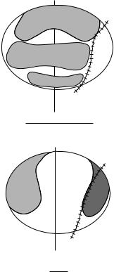
During knee flexion, the patella makes a rolling/gliding motion along the femoral articulating surface. Throughout the entire flexion range, the gliding motion is clockwise (Figure 3.12). In contrast, the direction of the rolling motion is counter-clockwise between 0 and 90◦ and clockwise between 90 and
S |
|
90 |
A |
L |
M |
45 |
|
20 |
|
|
B |
20° 45° |
90° |
S |
|
|
A |
L |
M |
|
B
135°
FIGURE 3.10 Diagrammatic representation of patella contact areas for varying degrees of knee flexion. (From Goodfellow J., Hungerford D.S., and Zindel M. J. Bone Joint Surg. 58-B: 3, 288. With permission.)