

Biomechanics Principles and Applications - Donald R. Peterson & Joseph D. Bronzino
.pdf1-6 |
Biomechanics |
equation that yields the following relationship involving the stiffness matrix:
ρV 2Um = Cmrns Nr Ns Un |
(1.9) |
where ρ is the density of the medium, V is the wave speed, and U and N are unit vectors along the particle displacement and wave propagation directions, respectively, so that Um, Nr , etc. are direction cosines.
Thus to find the five transverse isotropic elastic constants, at least five independent measurements are required, for example, a dilatational longitudinal wave in the 2 and 1(2) directions, a transverse wave in the 13(23) and 12 planes, etc. The technical moduli must then be calculated from the full set of Cij. For improved statistics, redundant measurements should be made. Correspondingly, for orthotropic symmetry, enough independent measurements must be made to obtain all 9 Cij; again, redundancy in measurements is a suggested approach.
One major advantage of the ultrasonic measurements over mechanical testing is that the former can be done with specimens too small for the latter technique. Second, the reproducibility of measurements using the former technique is greater than for the latter. Still a third advantage is that the full set of either five or nine coefficients can be measured on one specimen, a procedure not possible with the latter techniques. Thus, at present, most of the studies of elastic anisotropy in both human and other mammalian bone are done using ultrasonic techniques. In addition to the bulk wave type measurements described above, it is possible to obtain Young’s modulus directly. This is accomplished by using samples of small cross sections with transducers of low frequency so that the wavelength of the sound is much larger than the specimen size. In this case, an extensional longitudinal (bar) wave is propagated (which experimentally is analogous to a uniaxial mechanical test experiment), yielding
V 2 = |
E |
(1.10) |
ρ |
This technique was used successfully to show that bovine plexiform bone was definitely orthotropic while bovine haversian bone could be treated as transversely isotropic [Lipson and Katz, 1984]. The results were subsequently confirmed using bulk wave propagation techniques with considerable redundancy [Maharidge, 1984].
Table 1.2 lists the Cij (in GPa) for human (haversian) bone and bovine (both haversian and plexiform) bone. With the exception of Knets’ [1978] measurements, which were made using quasi-static mechanical testing, all the other measurements were made using bulk ultrasonic wave propagation.
In Maharidge’s study [1984], both types of tissue specimens, haversian and plexiform, were obtained from different aspects of the same level of an adult bovine femur. Thus the differences in Cij reported between the two types of bone tissue are hypothesized to be due essentially to the differences in
TABLE 1.2 Elastic Stiffness Coefficients for Various Human and Bovine Bones
Experiments |
C11 |
C22 |
C33 |
C44 |
C55 |
C66 |
C12 |
C13 |
C23 |
(bone type) |
(GPa) (GPa) (GPa) (GPa) (GPa) (GPa) |
(GPa) |
(GPa) |
(GPa) |
|||||
|
|
|
|
|
|
|
|
|
|
Van Buskirk and Ashman |
14.1 |
18.4 |
25.0 |
7.00 |
6.30 |
5.28 |
6.34 |
4.84 |
6.94 |
[1981] (bovine femur) |
|
|
|
|
|
|
|
|
|
Knets [1978] (human tibia) |
11.6 |
14.4 |
22.5 |
4.91 |
3.56 |
2.41 |
7.95 |
6.10 |
6.92 |
Van Buskirk and Ashman |
20.0 |
21.7 |
30.0 |
6.56 |
5.85 |
4.74 |
10.9 |
11.5 |
11.5 |
[1981] (human femur) |
|
|
|
|
|
|
|
|
|
Maharidge [1984] |
21.2 |
21.0 |
29.0 |
6.30 |
6.30 |
5.40 |
11.7 |
12.7 |
11.1 |
(bovine femur haversian) |
|
|
|
|
|
|
|
|
|
Maharidge [1984] |
22.4 |
25.0 |
35.0 |
8.20 |
7.10 |
6.10 |
14.0 |
15.8 |
13.6 |
(bovine femur plexiform) |
|
|
|
|
|
|
|
|
|
|
|
|
|
|
|
|
|
|
|
All measurements made with ultrasound except for Knets [1978] mechanical tests.

Mechanics of Hard Tissue |
1-7 |
(a) |
(b) |
L |
L |
|
R |
R |
|
|
|
T |
|
T |
|
|
FIGURE 1.3 Diagram showing how laminar (plexiform) bone (a) differs more between radial and tangential directions (R and T ) than does haversian bone (b). The arrows are vectors representing the various directions [Wainwright et al., 1982]. (Courtesy Princeton University Press.)
microstructural organization (Figure 1.3) [Wainwright et al., 1982]. The textural symmetry at this level of structure has dimensions comparable to those of the ultrasound wavelengths used in the experiment, and the molecular and ultrastructural levels of organization in both types of tissues are essentially identical. Note that while C11 almost equals C22 and that C44 and C55 are equal for bovine haversian bone, C11 and C22 and C44 and C55 differ by 11.6 and 13.4%, respectively, for bovine plexiform bone. Similarly, although C66 and 12 (C11 − C12) differ by 12.0% for the haversian bone, they differ by 31.1% for plexiform bone. Only the differences between C13 and C23 are somewhat comparable: 12.6% for haversian bone and 13.9% for plexiform. These results reinforce the importance of modeling bone as a hierarchical ensemble in order to understand the basis for bone’s elastic properties as a composite material-structure system in which the collagen–Ap components define the material composite property. When this material property is entered into calculations based on the microtextural arrangement, the overall anisotropic elastic anisotropy can be modeled.
The human femur data [Van Buskirk and Ashman, 1981] support this description of bone tissue. Although they measured all nine individual Cij, treating the femur as an orthotropic material, their results are consistent with a near transverse isotropic symmetry. However, their nine Cij for bovine femoral bone clearly shows the influence of the orthotropic microtextural symmetry of the tissue’s plexiform structure.
The data of Knets [1978] on human tibia are difficult to analyze. This could be due to the possibility of significant systematic errors due to mechanical testing on a large number of small specimens from a multitude of different positions in the tibia.
The variations in bone’s elastic properties cited earlier above due to location is appropriately illustrated in Table 1.3, where the mean values and standard deviations (all in GPa) for all g orthotropic Cij are given for bovine cortical bone at each aspect over the entire length of bone.
Since the Cij are simply related to the “technical” elastic moduli, such as Young’s modulus (E ), shear modulus (G ), bulk modulus (K ), and others, it is possible to describe the moduli along any given direction. The full equations for the most general anisotropy are too long to present here. However, they can be found in Yoon and Katz [1976a]. Presented below are the simplified equations for the case of transverse isotropy. Young’s modulus is
1 |
|
S |
|
1 |
|
γ 2 |
2S |
|
γ 4 S |
|
γ 2 |
1 |
|
γ 2 |
(2S |
|
S |
|
) |
(1.11) |
|
E (γ3) = |
= |
− |
11 + |
33 + |
− |
13 + |
44 |
||||||||||||||
33 |
|
3 |
|
3 |
3 |
|
3 |
|
|
|
|||||||||||
where γ3 = cos φ, and φ is the angle made with respect to the bone (3) axis.
1-8 |
|
|
|
|
Biomechanics |
|
|
TABLE 1.3 Mean Values and Standard Deviations for the Cij Measured by Van Buskirk and |
|||||
|
Ashman [1981] at Each Aspect Over the Entire Length of Bone (all Values in GPa) |
|
|
|||
|
|
|
|
|
|
|
|
|
Anterior |
Medial |
Posterior |
Lateral |
|
|
|
|
|
|
|
|
|
C11 |
18.7 ± 1.7 |
20.9 ± 0.8 |
20.1 ± 1.0 |
20.6 ± 1.6 |
|
|
C22 |
20.4 ± 1.2 |
22.3 ± 1.0 |
22.2 ± 1.3 |
22.0 ± 1.0 |
|
|
C33 |
28.6 ± 1.9 |
30.1 ± 2.3 |
30.8 ± 1.0 |
30.5 ± 1.1 |
|
|
C44 |
6.73 ± 0.68 |
6.45 ± 0.35 |
6.78 ± 1.0 |
6.27 ± 0.28 |
|
|
C55 |
5.55 ± 0.41 |
6.04 ± 0.51 |
5.93 ± 0.28 |
5.68 ± 0.29 |
|
|
C66 |
4.34 ± 0.33 |
4.87 ± 0.35 |
5.10 ± 0.45 |
4.63 ± 0.36 |
|
|
C12 |
11.2 ± 2.0 |
11.2 ± 1.1 |
10.4 ± 1.0 |
10.8 ± 1.7 |
|
|
C13 |
11.2 ± 1.1 |
11.2 ± 2.4 |
11.6 ± 1.7 |
11.7 ± 1.8 |
|
|
C23 |
10.4 ± 1.4 |
11.5 ± 1.0 |
12.5 ± 1.7 |
11.8 ± 1.1 |
|
The shear modulus (rigidity modulus or torsional modulus for a circular cylinder) is
|
|
1 |
|
|
= |
1 |
|
S |
|
S |
|
= |
S |
44 + |
(S |
11 − |
S |
|
) |
|
1 |
S |
|
1 |
− |
γ 2 |
|||||
|
G (γ3) |
|
|
|
|
|
|
|
|
|
|||||||||||||||||||||
|
2 |
|
44 + |
|
55 |
|
|
|
12 |
|
− 2 |
44 |
|
3 |
|||||||||||||||||
|
|
|
|
|
|
+ 2(S11 + S33 − 2S13 − S44)γ32 1 − γ32 |
|
|
|
|
|||||||||||||||||||||
where, again γ3 = cos φ. |
|
|
|
|
|
|
|
|
|
|
|
|
|
|
|
|
|
|
|
|
|
|
|
|
|
|
|
|
|
||
The bulk modulus (reciprocal of the volume compressibility) is |
|
|
|
|
|
|
|
||||||||||||||||||||||||
1 |
= |
S |
33 |
+ |
2(S |
11 + |
S |
12 |
+ |
2S |
13 |
) |
= |
|
C11 + C12 + 2C33 − 4C13 |
||||||||||||||||
|
K |
C33(C11 + C12) − 2C132 |
|||||||||||||||||||||||||||||
|
|
|
|
|
|
|
|
|
|||||||||||||||||||||||
(1.12)
(1.13)
Conversion of Equation 1.11 and Equation 1.12 from Sij to Cij can be done by using the following transformation equations:
|
|
S11 |
= |
C22C33 |
− C232 |
|
S22 |
= |
C33C11 |
− C132 |
|
|
|
||||||||
|
|
C11C22 |
− C122 |
|
C13C23 |
− C12C33 |
|||||||||||||||
|
|
S33 |
= |
|
S12 |
= |
|
|
|||||||||||||
|
|
|
C12C23 |
|
|
|
|
|
C12C13 − C23C11 |
||||||||||||
|
|
S13 |
= |
− C13C22 |
|
S23 = |
|
||||||||||||||
|
|
|
|
|
|
|
|
||||||||||||||
|
|
|
|
1 |
|
|
|
1 |
|
|
1 |
|
(1.14) |
||||||||
|
|
S44 |
= |
|
|
|
S55 = |
|
|
|
S66 = |
|
|
||||||||
|
|
|
C44 |
C55 |
|
|
C66 |
||||||||||||||
where |
|
|
|
|
|
|
|
|
|
|
|
|
|
|
|
|
|
|
|
|
|
C11 |
C12 |
C13 |
|
|
|
|
|
|
|
|
|
|
|
|
|
|
|
|
|
|
|
= C12 |
C22 |
C23 |
= C11C22C33 |
+ 2C12C23C13 − C11C232 + C22C132 + C33C122 (1.15) |
|||||||||||||||||
C13 |
C23 |
C33 |
|
|
|
|
|
|
|
|
|
|
|
|
|
|
|
|
|
|
|
In addition to data on the elastic properties of cortical bone presented above, there is also available a considerable set of data on the mechanical properties of cancellous (trabecullar) bone including measurements of the elastic properties of single trabeculae. Indeed as early as 1993, Keaveny and Hayes [1993] presented an analysis of 20 years of studies on the mechanical properties of trabecular bone. Most of the earlier studies used mechanical testing of bulk specimens of a size reflecting a cellular solid, that is, of the order of cubic mm or larger. These studies showed that both the modulus and strength of trabecular bone are strongly correlated to the apparent density, where apparent density, ρa, is defined as the product of individual trabeculae density, ρt, and the volume fraction of bone in the bulk specimen, Vf, and is given by ρa = ρt Vf.

Mechanics of Hard Tissue |
|
|
1-9 |
||
|
TABLE 1.4 Elastic Moduli of Trabecular Bone Material Measured by |
||||
|
Different Experimental Methods |
|
|
|
|
|
|
|
|
|
|
|
|
|
Average |
|
|
|
Study |
Method |
Modulus |
(GPa) |
|
|
|
|
|
|
|
|
Townsend et al. [1975] |
Buckling |
11.4 |
(Wet) |
|
|
|
Buckling |
14.1 |
(Dry) |
|
|
Ryan and Williams [1989] |
Uniaxial tension |
0.760 |
|
|
|
Choi et al. [1992] |
4-point bending |
5.72 |
|
|
|
Ashman and Rho [1988] |
Ultrasound |
13.0 |
(Human) |
|
|
|
Ultrasound |
10.9 |
(Bovine) |
|
|
Rho et al. [1993] |
Ultrasound |
14.8 |
|
|
|
|
Tensile test |
10.4 |
|
|
|
Rho et al. [1999] |
Nanoindentation |
19.4 |
(Longitudinal) |
|
|
|
Nanoindentation |
15.0 |
(Transverse) |
|
|
Turner et al. [1999] |
Acoustic microscopy |
17.5 |
|
|
|
|
Nanoindentation |
18.1 |
|
|
|
Bumrerraj and Katz [2001] |
Acoustic microscopy |
17.4 |
|
|
|
|
|
|
|
|
Elastic moduli, E , from these measurements generally ranged from approximately 10 MPa to the order of 1 GPa depending on the apparent density and could be correlated to the apparent density in g/cc by a power law relationship, E = 6.13Pa144, calculated for 165 specimens with an r 2 = 0.62 [Keaveny and Hayes, 1993].
With the introduction of micromechanical modeling of bone, it became apparent that in addition to knowing the bulk properties of trabecular bone it was necessary to determine the elastic properties of the individual trabeculae. Several different experimental techniques have been used for these studies. Individual trabeculae have been machined and measured in buckling, yielding a modulus of 11.4 GPa (wet) and 14.1 GPa (dry) [Townsend et al., 1975], as well as by other mechanical testing methods providing average values of the elastic modulus ranging from less than 1 GPa to about 8 GPa (Table 1.4). Ultrasound measurements [Ashman and Rho, 1988; Rho et al., 1993] have yielded values commensurate with the measurements of Townsend et al. [1975] (Table 1.4). More recently, acoustic microscopy and nanoindentation have been used, yielding values significantly higher than those cited above. Rho et al. [1999] using nanoindentation obtained average values of modulus ranging from 15.0 to 19.4 GPa depending on orientation, as compared to 22.4 GPa for osteons and 25.7 GPa for the interstitial lamellae in cortical bone (Table 1.4). Turner et al. [1999] compared nanoindentation and acoustic microscopy at 50 MHz on the same specimens of trabecular and cortical bone from a common human donor. While the nanoindentation resulted in Young’s moduli greater than those measured by acoustic microscopy by 4 to 14%, the anisotropy ratio of longitudinal modulus to transverse modulus for cortical bone was similar for both modes of measurement; the trabecular values are given in Table 1.4. Acoustic microscopy at 400 MHz has also been used to measure the moduli of both human trabecular and cortical bone [Bumrerraj and Katz, 2001], yielding results comparable to those of Turner et al. [1999] for both types of bone (Table 1.4).
These recent studies provide a framework for micromechanical analyses using material properties measured on the microstructural level. They also point to using nano-scale measurements, such as those provided by atomic force microscopy (AFM), to analyze the mechanics of bone on the smallest unit of structure shown in Figure 1.1.
1.4 Characterizing Elastic Anisotropy
Having a full set of five or nine Cij does permit describing the anisotropy of that particular specimen of bone, but there is no simple way of comparing the relative anisotropy between different specimens of the same bone or between different species or between experimenters’ measurements by trying to relate individual Cij between sets of measurements. Adapting a method from crystal physics [Chung and Buessem, 1968] Katz and Meunier [1987] presented a description for obtaining two scalar quantities defining the
1-10 |
|
|
|
Biomechanics |
|
TABLE 1.5 Ac (%) vs. As (%) for Various Types of Hard |
|||
|
Tissues and Apatites |
|
|
|
|
|
|
|
|
|
Experiments (specimen type) |
Ac (%) As (%) |
||
|
Van Buskirk et al. [1981] (bovine femur) |
1.522 |
2.075 |
|
|
Katz and Ukraincik [1971] (OHAp) |
0.995 |
0.686 |
|
|
Yoon (redone) in Katz [1984] (FAp) |
0.867 |
0.630 |
|
|
Lang [1969,1970] (bovine femur dried) |
1.391 |
0.981 |
|
|
Reilly and Burstein [1975] (bovine femur) |
2.627 |
5.554 |
|
|
Yoon and Katz [1976] (human femur dried) |
1.036 |
1.055 |
|
|
Katz et al. [1983] (haversian) |
1.080 |
0.775 |
|
|
Van Buskirk and Ashman [1981] (human femur) |
1.504 |
1.884 |
|
|
Kinney et al. [2004] (human dentin dry) |
0.006 |
0.011 |
|
|
Kinney et al. [2004] (human dentin wet) |
1.305 |
0.377 |
|
|
|
|
|
|
compressive and shear anisotropy for bone with transverse isotropic symmetry. Later, they developed a similar pair of scalar quantities for bone exhibiting orthotropic symmetry [Katz and Meunier, 1990]. For both cases, the percentage compressive ( Ac ) and shear (As ) elastic anisotropy are given, respectively, by
Ac (%) |
= |
100 |
|
K V − KR |
|
|
K V + KR |
|
|||||
|
|
|
|
|||
As (%) |
= |
100 |
G V − G R |
|
(1.16) |
|
|
||||||
|
|
|
G V + G R |
|||
where K V and KR are the Voigt (uniform strain across an interface) and Reuss (uniform stress across an interface) bulk moduli, respectively, and G V and G R are the Voigt and Reuss shear moduli, respectively. The equations for K V, KR, G V, and G R are provided for both transverse isotropy and orthotropic symmetry in Appendix.
Table 1.5 lists the values of As (%) and Ac (%) for various types of hard tissues and apatites. The graph of As (%) vs. Ac (%) is given in Figure 1.4.
As (%) and Ac (%) have been calculated for a human femur, having both transverse isotropic and orthotropic symmetry, from the full set of Van Buskirk and Ashman [1981] Cij data at each of the four aspects around the periphery, anterior, medial, posterior, and lateral, as denoted in Table 1.3, at fractional proximal levels along the femur’s length, Z/L = 0.3 to 0.7. The graph of As (%) vs. Z/L , assuming transverse isotropy, is given in Figure 1.5. Note that the Anterior aspect, that is in tension during loading,
|
|
|
|
|
|
|
|
|
|
|
|
|
|
|
|
|
|
3.5 |
|
(%)*Asvs.Ac*(%)for |
varioustypesofhard |
tissuesandapatites |
|
|
|
|
|
|
|
|
|
|
|
|
|
|
|
3.0 |
|
047e=0. |
R |
|
|
|
|
|
|
|
|
|
|
|
|
|
1.50.0 1.5 2.0 2.5 |
Ac*(%) |
|||
|
|
|
2.194x |
=0.767 |
|
|
|
|
|
|
|
|
|
|
|
|
|
|
|
|
|
|
|
2 |
|
|
|
|
|
|
|
|
|
|
|
|
|
|
|
|
|
|
y |
|
|
|
|
|
|
|
|
|
|
|
|
|
|
0.0 |
|
|
|
8.0 |
7.5 |
7.0 |
|
6.0 |
|
5.0 |
4.5 |
|
|
3.0 |
2.5 |
|
|
|
|
|
|
|
|
6.5 |
5.5 |
4.0 |
3.5 |
2.0 |
1.5 |
1.0 |
0.5 |
0.0 |
|
||||||||
|
|
|
|
|
|
|
|
|
|
As* (%) |
|
|
|
|
|
|
|
|
|
FIGURE 1.4 Values of As (%) vs. Ac (%) from Table 1.5 are plotted for various types of hard tissues and apatites.

Mechanics of Hard Tissue |
1-11 |
As* (%) vs. Z/L for transverse Isotropic
|
6.0 |
|
5.0 |
|
4.0 |
*(%) |
3.0 |
As |
|
|
2.0 |
|
1.0 |
|
0.0 |
Anterior
 Posterior
 Medial
 Lateral
0.3 |
0.4 |
0.5 |
0.6 |
0.7 |
|
|
Z/L |
|
|
FIGURE 1.5 Calculated values of As (%) for human femoral bone, treated as having transverse isotropic symmetry, is plotted vs. Z/L for all four aspects, anterior, medial, posterior, lateral around the bone’s periphery; Z/L is the fractional proximal distance along the femur’s length.
has values of As (%) in some positions considerably higher than those of the other aspects. Similarly, the graph of Ac (%) vs. Z/L is given in Figure 1.6. Note here it is the posterior aspect that is in compression during loading, which has values of Ac (%) in some positions considerably higher than those of the other aspects. Both graphs are based on the transverse isotropic symmetry calculations; however, the identical trends were obtained based on the orthotropic symmetry calculations. It is clear that in addition to the moduli varying along the length and over all four aspects of the femur, the anisotropy varies as well, reflecting the response of the femur to the manner of loading.
Recently, Kinney et al. [2004] used the technique of resonant ultrasound spectroscopy (RUS) to measure the elastic constants (Cij) of human dentin from both wet and dry samples. As (%) and Ac (%) calculated from these data are included in both Table 1.5 and Figure 1.4. Their data showed that the samples exhibited transverse isotropic symmetry. However, the Cij for dry dentin implied even higher symmetry. Indeed, the result of using the average value for C11 and C12 = 36.6 GPa and the value for C44 = 14.7 GPa for dry
Ac* (%)
As* (%) vs. Z/L for transverse Isotropic
6.0
5.0 |
|
|
|
|
4.0 |
|
|
|
Anterior |
|
|
|
|
|
3.0 |
|
|
|
Posterior |
|
|
|
Medial |
|
|
|
|
|
|
2.0 |
|
|
|
Lateral |
|
|
|
|
|
1.0 |
|
|
|
|
0.0 |
|
|
|
|
0.3 |
0.4 |
0.5 |
0.6 |
0.7 |
Z/L
FIGURE 1.6 Calculated values of Ac (%) for human femoral bone, treated as having transverse isotropic symmetry, is plotted vs. Z/L for all four aspects, anterior, medial, posterior, lateral around the bone’s periphery; Z/L is the fractional proximal distance along the femur’s length.

1-12 |
Biomechanics |
dentin in the calculations suggests that dry human dentin is very nearly elastically isotropic. This isotropiclike behavior of the dry dentin may have clinical significance. There is independent experimental evidence to support this calculation of isotropy based on the ultrasonic data. Small angle x-ray diffraction of human dentin yielded results implying isotropy near the pulp and mild anisotropy in mid-dentin [Kinney et al., 2001].
It is interesting to note that haversian bones, whether human or bovine, have both their compressive and shear anisotropy factors considerably lower than the respective values for plexiform bone. Thus, not only is plexiform bone both stiffer and more rigid than haversian bone, it is also more anisotropic. These two scalar anisotropy quantities also provide a means of assessing whether there is the possibility either of systematic errors in the measurements or artifacts in the modeling of the elastic properties of hard tissues. This is determined when the values of Ac (%) and/or As (%) are much greater than the close range of lower values obtained by calculations on a variety of different ultrasonic measurements (Table 1.5). A possible example of this is the value of As (%) = 7.88 calculated from the mechanical testing data of Knets [1978], Table 1.2.
1.5 Modeling Elastic Behavior
Currey [1964] first presented some preliminary ideas of modeling bone as a composite material composed of a simple linear superposition of collagen and Ap. He followed this later [1969] with an attempt to take into account the orientation of the Ap crystallites using a model proposed by Cox [1952] for fiber-reinforced composites. Katz [1971a] and Piekarski [1973] independently showed that the use of Voigt and Reuss or even Hashin–Shtrikman [1963] composite modeling showed the limitations of using linear combinations of either elastic moduli or elastic compliances. The failure of all these early models could be traced to the fact that they were based only on considerations of material properties. This is comparable to trying to determine the properties of an Eiffel Tower built using a composite material by simply modeling the composite material properties without considering void spaces and the interconnectivity of the structure [Lakes, 1993]. In neither case is the complexity of the structural organization involved. This consideration of hierarchical organization clearly must be introduced into the modeling.
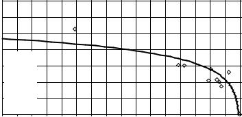
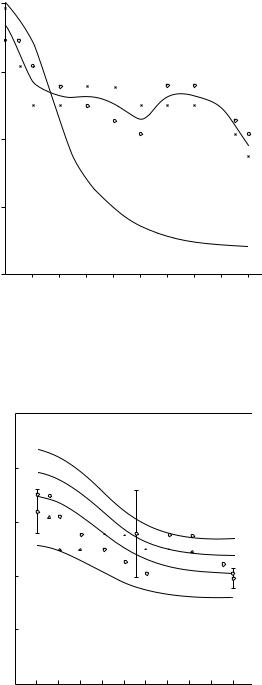
Katz in a number of papers [1971b, 1976] and meeting presentations put forth the hypothesis that haversian bone should be modeled as a hierarchical composite, eventually adapting a hollow fiber composite model by Hashin and Rosen [1964]. Bonfield and Grynpas [1977] used extensional (longitudinal) ultrasonic wave propagation in both wet and dry bovine femoral cortical bone specimens oriented at angles of 5, 10, 20, 40, 50, 70, 80, and 85◦ with respect to the long bone axis. They compared their experimental results for Young’s moduli with the theoretical curve predicted by Currey’s model [1969]; this is shown in Figure 1.7. The lack of agreement led them to “conclude, therefore that an alternative model is required to account for the dependence of Young’s modulus on orientation” [Bonfield and Grynpas, 1977]. Katz [1980, 1981], applying his hierarchical material-structure composite model, showed that the data in Figure 1.7 could be explained by considering different amounts of Ap crystallites aligned parallel to the long bone axis; this is shown in Figure 1.8. This early attempt at hierarchical micromechanical modeling is now being extended with more sophisticated modeling using either finite-element micromechanical computations [Hogan, 1992] or homogenization theory [Crolet et al., 1993]. Further improvements will come by including more definitive information on the structural organization of collagen and Ap at the molecular-ultrastructural level [Wagner and Weiner, 1992; Weiner and Traub, 1989].
1.6 Viscoelastic Properties
As stated earlier, bone (along with all other biologic tissues) is a viscoelastic material. Clearly, for such materials, Hooke’s law for linear elastic materials must be replaced by a constitutive equation that includes the time dependency of the material properties. The behavior of an anisotropic linear viscoelastic material
Mechanics of Hard Tissue |
1-13 |
) –2
E m(GN
20
15
10
5
20
10 |
20 |
30 |
40 |
50 |
60 |
70 |
80 |
90 |
Orientation (degrees)
FIGURE 1.7 Variation in Young’s modulus of bovine femur specimens (E ) with the orientation of specimen axis to the long axis of the bone, for wet (o) and dry (x) conditions compared with the theoretical curve (———) predicted from a fiber-reinforced composite model [Bonfield and Grynpas, 1977]. (Courtesy Nature 1977, 270: 453. ©Macmillan Magazines Ltd.)
) 2 (GN/mmodulus
Young’s
25
A
20 |
B |
|
|
||
|
C |
|
15 |
|
|
|
D |
|
10 |
|
|
5 |
Longitudianl fibers |
|
A=64% |
||
|
||
|
B=57% |
|
|
C=50% |
|
|
D=37% |
0
0° 10° 20° 30° 40° 50° 60° 70° 80° 90° Orientation of sample relative to longitudinal axis of model and bone ( =cos–1 )
FIGURE 1.8 Comparison of predictions of Katz two-level composite model with the experimental data of Bonfield and Grynpas. Each curve represents a different lamellar configuration within a single osteon, with longitudinal fibers; A, 64%; B, 57%; C, 50%; D, 37%; and the rest of the fibers assumed horizontal. (From Katz J.L., Mechanical Properties of Bone, AMD, vol. 45, New York, American Society of Mechanical Engineers, 1981. With permission.)
1-14 |
Biomechanics |
may be described by using the Boltzmann superposition integral as a constitutive equation:
|
t |
d kl (τ ) |
|
|
|
σij(t) = |
Cijkl(t − τ ) |
dτ |
(1.17) |
||
dτ |
|||||
|
−∞ |
|
|
|
where σij(t) and kl (τ ) are the time-dependent second-rank stress and strain tensors, respectively, and Cijkl(t − τ ) is the fourth-rank relaxation modulus tensor. This tensor has 36 independent elements for the lowest symmetry case and 12 nonzero independent elements for an orthotropic solid. Again, as for linear elasticity, a reduced notation is used, that is, 11 → 1, 22 → 2, 33 → 3, 23 → 4, 31 → 5, and 12 → 6. If we apply Equation 1.17 to the case of an orthotropic material, for example, plexiform bone, in uniaxial tension (compression) in the one direction [Lakes and Katz, 1974], in this case using the reduced notation, we obtain
|
t |
|
d 1(τ ) |
|
|
|
d 2(τ ) |
|
|
|
d 3(τ ) |
|
|
||||||||
σ1(t) = |
C11(t − |
τ ) |
+ C12 |
(t − |
τ ) |
+ C13 |
(t − |
τ ) |
dτ |
(1.18) |
|||||||||||
dτ |
|
|
dτ |
|
dτ |
|
|||||||||||||||
|
−∞ |
|
|
|
|
|
|
|
|
|
|
|
|
|
|
|
|
|
|
|
|
|
t |
|
d 1(τ ) |
|
|
|
d 2(τ ) |
|
|
|
d 3(τ ) |
|
|
||||||||
σ2(t) = |
C21(t − |
τ ) |
+ C22 |
(t − |
τ ) |
+ C23 |
(t − |
τ ) |
= 0 |
(1.19) |
|||||||||||
dτ |
|
|
dτ |
|
dτ |
|
|||||||||||||||
|
−∞ |
|
|
|
|
|
|
|
|
|
|
|
|
|
|
|
|
|
|
|
|
for all t, and |
|
|
|
|
|
|
|
|
|
|
|
|
|
|
|
|
|
|
|
|
|
|
t |
d 1(τ ) |
|
|
|
|
d 2(τ ) |
|
|
|
d 3(τ ) |
|
|
|
|||||||
σ3(t) = |
C31(t − τ ) |
+ C32(t − τ ) |
+ C33(t − τ ) |
dτ = 0 |
(1.20) |
||||||||||||||||
dτ |
|
dτ |
|
dτ |
|
||||||||||||||||
−∞ |
|
|
|
|
|
|
|
|
|
|
|
|
|
|
|
|
|
|
|
||
for all t.
Having the integrands vanish provides an obvious solution to Equation 1.19 and Equation 1.20. Solving them simultaneously for [d 2(τ )]/dτ and [d 3(τ )]/dτ and substituting these values in Equation 1.17 yields
|
|
|
|
|
|
|
|
|
|
|
|
t |
|
d 1(τ ) |
|
||||||
|
|
|
|
|
|
|
|
|
|
|
|
|
|
(1.21) |
|||||||
|
|
|
|
|
|
|
|
|
|
σ1(t) = |
|
E 1(t − τ ) |
|
|
|
dτ |
|||||
|
|
|
|
|
|
|
|
|
|
−∞ |
|
dτ |
|
||||||||
|
|
|
|
|
|
|
|
|
|
|
|
|
|
|
|
|
|
|
|
||
where, if for convenience we adopt the notation Cij ≡ Cij(t − τ ), then Young’s modulus is given by |
|||||||||||||||||||||
E |
|
(t |
− |
τ ) |
= |
C |
|
+ |
C |
|
[C31 − (C21C33/C23)] |
+ |
C |
|
|
[C21 − (C31C22/C32)] |
(1.22) |
||||
1 |
11 |
12 [(C21C33/C23) − C32] |
13 [(C22C33/C32)/ − C23] |
||||||||||||||||||
|
|
|
|
|
|
||||||||||||||||
In this case of uniaxial tension (compression), only nine independent orthotropic tensor components are involved, the three shear components being equal to zero. Still, this time-dependent Young’s modulus is a rather complex function. As in the linear elastic case, the inverse form of the Boltzmann integral can be used; this would constitute the compliance formulation.
If we consider the bone being driven by a strain at a frequency ω, with a corresponding sinusoidal stress lagging by an angle δ, then the complex Young’s modulus E (ω) may be expressed as
E (ω) |
= |
E (ω) |
+ |
iE (ω) |
(1.23) |
|
|
|
Mechanics of Hard Tissue |
1-15 |
where E (ω), which represents the stress–strain ratio in phase with the strain, is known as the storage modulus, and E (ω), which represents the stress–strain ratio 90 degrees out of phase with the strain, is known as the loss modulus. The ratio of the loss modulus to the storage modulus is then equal to tan δ. Usually, data are presented by a graph of the storage modulus along with a graph of tan δ, both against frequency. For a more complete development of the values of E (ω) and E (ω), as well as for the derivation of other viscoelastic technical moduli, see Lakes and Katz [1974]; for a similar development of the shear storage and loss moduli, see Cowin [1989].
Thus, for a more complete understanding of bone’s response to applied loads, it is important to know its rheologic properties. There have been a number of early studies of the viscoelastic properties of various long bones [Sedlin, 1965; Smith and Keiper, 1965; Lugassy, 1968; Black and Korostoff, 1973; Laird and Kingsbury, 1973]. However, none of these was performed over a wide enough range of frequency (or time) to completely define the viscoelastic properties measured, for example, creep or stress relaxation. Thus it is not possible to mathematically transform one property into any other to compare results of three different experiments on different bones [Lakes and Katz, 1974].
In the first experiments over an extended frequency range, the biaxial viscoelastic as well as uniaxial viscoelastic properties of wet cortical human and bovine femoral bone were measured using both dynamic and stress relaxation techniques over eight decades of frequency (time) [Lakes et al., 1979]. The results of these experiments showed that bone was both nonlinear and thermorheologically complex, that is, time–temperature superposition could not be used to extend the range of viscoelastic measurements. A nonlinear constitutive equation was developed based on these measurements [Lakes and Katz, 1979a].
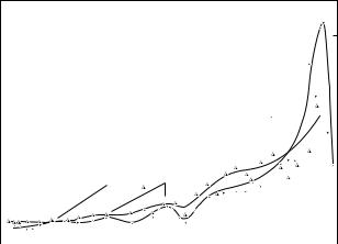
In addition, relaxation spectrums for both human and bovine cortical bone were obtained; Figure 1.9 shows the former [Lakes and Katz, 1979b]. The contributions of several mechanisms to the loss tangent of cortical bone is shown in Figure 1.10 [Lakes and Katz, 1979b]. It is interesting to note that almost all the major loss mechanisms occur at frequencies (times) at or close to those in which there are “bumps,” indicating possible strain energy dissipation, on the relaxation spectra shown on Figure 1.9. An extensive review of the viscoelastic properties of bone can be found in the CRC publication Natural and Living Biomaterials [Lakes and Katz, 1984].
0.06
|
|
|
|
|
|
|
|
|
|
|
|
|
|
|
|
|
|
|
|
|
|
|
|
|
0.04 |
H (τ) |
|
|
|
|
|
|
|
|
|
|
|
|
|
|
|
|
|
|
|
|
|
|
|
|
|||
|
|
|
|
|
|
|
|
|
|
|
|
|
|
|
|
|
|
|
|
|
|
|
|
|
|
|
|
|
|
|
|
|
|
|
|
|
|
|
|
|
|
|
|
|
|
|
|
|
|
|
|
|
Gstd |
|
|
|
|
|
Lamellae |
Osteons |
|
|
|
|
|
|
|
|
|
|
|
0.02 |
|
|||||||
|
|
|
|
|
|
|
|
|
|
|
|
|
|
|
||||||||||||
|
|
|
|
|
|
|
|
|
|
|
|
|
|
|
|
|
|
|
|
|
||||||
|
|
|
|
|
|
|
|
|
|
|
|
|
|
|
|
|
|
|
|
|
|
|
|
|
0 |
|
|
|
|
|
|
|
|
|
|
|
|
|
|
|
|
|
|
|
|
|
|
|
|
|
|
||
10–3 |
10–2 |
10–1 |
1 |
10 |
102 |
103 |
104 |
105 |
|
|||||||||||||||||
|
|
|
|
|
|
|
|
|
|
|
, sec |
|
|
|
|
|
|
|
|
|
|
|
|
|
||
FIGURE 1.9 Comparison of relaxation spectra for wet human bone, specimens 5 and 6 [Lakes et al., 1979] in simple torsion; T = 37◦ C. First approximation from relaxation and dynamic data. • Human tibial bone, specimen 6. Human tibial bone, specimen 5, G std = G (10 sec). G std(5) = G (10 sec). G std(5) = 0.590 × 10⁶ lb/in2. G std(6) × 0.602 × 106 lb/in2. (Courtesy Journal of Biomechanics, Pergamon Press.)