

Computational Methods for Protein Structure Prediction & Modeling V1 - Xu Xu and Liang
.pdf370 |
Jianpeng Ma |
Fig. 11.10 A new deconvolution method. (a) A simple 2D example of deconvolution. The left is
the original image, the middle is the image rendered with noises, and the right is the deconvoluted
˚ image. (b) A 3D example for deconvolution (right) on a piece of -sheet density blurred to 8 A
(left). The C -traces of the sheet (red) are superimposed on the density.
11.3.3A New Method for Deconvolution of Density Maps
In order to enhance the features of secondary structural elements in density maps for building pseudo-C -traces, we developed a new deconvolution method. An example is shown in Fig. 11.10a. A synthetic 2D geometrical object (left panel) was contaminated with a level of noise that nearly renders features in the original object indistinguishable (middle panel). Deconvolution resulted in a dramatic recovery of object features.
˚
The method was then tested on a simulated 3D density map blurred to 8 A (Fig. 11.10b, left). After deconvolution, strands are better resolved (Fig. 11.10b, right) and the subsequent building of pseudo-C -traces on the deconvoluted map became trivial.
The deconvolution method was then examined on experimental density maps of the 2 protein of reovirus. In order to have a more systematic and self-consistent test,
˚
the cryo-EM structures of reovirus were purposely reconstructed to 7.6-A resolution
˚
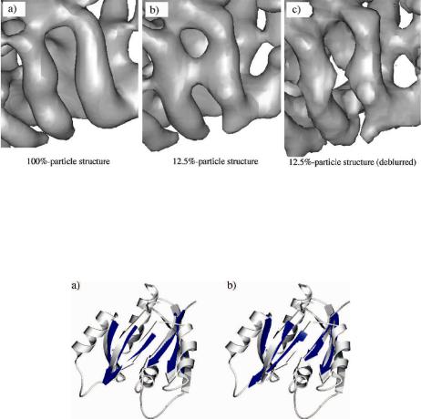
from 7939 single particle images (100%-particle structure) and to 11.8-A resolution from a subset (12.5%) of the same particle images (12.5%-particle structure). Two helices that are distinct in the 100%-particle structure (Fig. 11.11a) are bridged by density that interconnects the helices in the 12.5%-particle structure (presumably owing to the higher level of noise) (Fig. 11.11b). The deconvolution of the 12.5%- particle structure yields a map with distinct densities for the helices (Fig. 11.11c).
11.3.4Deconvolution and Trace Building in Simulated Density Maps of 12 Proteins
As demonstrated in previous sections, sheettracer can build pseudo-C -traces in
˚
simulated maps at resolutions as low as 6 A. To increase its effectiveness, the deconvolution method was combined with sheettracer to trace strands at lower resolutions.
Figure 11.12 shows the results of tracing with simulated maps of p21 |
ras |
˚ |
|
|
at 8 and 9 A. |
||
|
|
|
˚ |
The sensitivity, specificity, and rms deviations are 76.6%, 98.3%, and 1.65 A and |
|||
˚ |
˚ |
|
|
70.2%, 96.7%, and 1.73 A for 8 and 9 A, respectively. The methods were then applied
˚
to simulated density maps of the other 11 proteins at 8 A, and resulting average sen-
˚
sitivity, specificity, and rms deviations are 71.3%, 93.8%, and 1.77 A, respectively.
11. Intermediate-Resolution Density Maps |
371 |
Fig. 11.11 The improved appearance of secondary structural elements in the experimental density map of the 2 protein of reovirus by the deconvolution. (a) The cryo-EM structure generated using 100% particle images (100%-particle structure) highlighting the two well-separated helices. (b) The structure generated using 12.5% particle images (12.5%-particle structure) in which the two distinct helices are wrongfully connected. (c) The deconvolution procedure recovered the separation of these two helices in the 12.5%-particle structure.
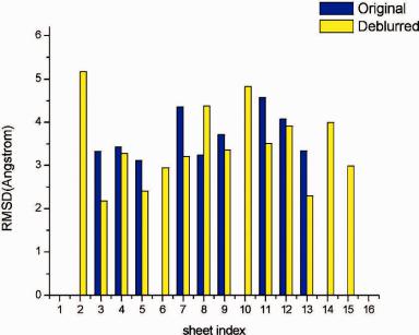
Fig. 11.12 Sheet-tracing results for p2l |
ras |
˚ |
˚ |
|
at resolutions of 8 A (a) and 9 A (b) after deconvolution. |
||
The built pseudo-C -traces of the sheets (blue) are shown on top of the ribbon diagrams of the crystal structure (lighter color).
These results clearly demonstrate that the deconvolution method can indeed enhance density interpretation by sheettracer.
11.3.5Deconvolution and Trace Building in Experimental Maps of Reovirus 2 Protein
To test sheetracer and the deconvolution method on real experimental data, we used
˚
the 7.6-A cryo-EM structure of the 2 protein of reovirus (Zhang et al., 2003), the crystal structure of which has been solved independently (Reinisch et al., 2000) (PDB code 1ej6) and could be used to validate the sheet-tracing results. The 2 protein has 16 -sheets, 12 of which contain three or more strands. The results of
372 |
Jianpeng Ma |
˚
Fig. 11.13 Comparison of sheet-tracing results in the 7.6-A density maps of the 2 protein of reovirus with (yellow bar) and without (blue bar) deconvolution. There are a total of 16 -sheets, 12 of which are large (three-stranded or more) and 4 are small (short two-stranded). In all cases except one (sheet 8), the deconvolution resulted in smaller rms deviations relative to the crystal structure than without. Moreover, the deconvolution brought up 5 additional -sheets (sheets 2, 6, 10, 14, and 15) for which no pseudo-C -traces could be built on the original maps without deconvolution.
building pseudo-C -traces with and without deconvolution are shown in Fig. 11.13. Except sheet 8, the deconvoluted maps always have better rms deviations of pseudo- C -traces compared with those obtained from the original map. Deconvolution also improved five additional sheets (sheets 2, 6, 10, 14, and 15) for which pseudo-C - traces could not be built from the original maps before deconvolution.
11.3.6Discussion
Not surprisingly, the accuracy of tracing generated by sheettracer depends at least in part on the reliability of sheetminer because the input to sheettracer consists of sheet density maps identified by sheetminer from raw density maps. Usually, the sensitivity of tracing is closely coupled to the performance of sheetminer, but the specificity of tracing is not and is always quite good. Moreover, similar to sheetminer, the size of-sheets also affects the performance of sheettracer. Sheetracer naturally performs better when the sheets are large and the strands are long because errors tend to occur near the edges of -sheets.
11. Intermediate-Resolution Density Maps |
373 |
Our results have shown that the deconvolution method significantly enhances one’s ability to build pseudo-C -traces for -strands at relatively low resolutions. However, it is hard to objectively and quantitatively measure the improvement on the effective resolution brought by the deconvolution method.
Computational methods for identifying and tracing secondary structural elements in intermediate-resolution density maps should be valuable for several reasons. First, the pseudo-C -traces will facilitate more biochemical and functional studies and will help structure refinement at higher resolutions. Second, the combination of sheettracer with other related computational methods (Elofsson et al., 1996; Jiang et al., 2001; Lu et al., 2002; Miller et al., 1996; Skolnick et al., 2001) will eventually make it possible to reveal protein folds from data at intermediate or lower resolutions. Third, the secondary structural elements established by sheettracer and related methods (Jiang et al., 2001) can provide guiding landmarks for docking atomic models of sub-components or homology-derived models into intermediate-resolution density maps. Accuracy of rigid-body docking should be significantly improved if even just a few points inside a density map can be reliably identified (Rossmann, 2000).
With sheetminer and sheettracer, the secondary structural skeletons can be deduced from intermediate-resolution density maps, but the topology, or the fold, remains unknown. Topology determination is the topic of the next section.
11.4Determining Protein Topology Based on Skeletons of Secondary Structures
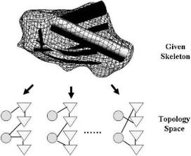
The output from programs like helixhunter (Jiang et al., 2001), sheetminer (Kong and Ma, 2003), and sheettracer (Kong et al., 2004) gives the locations of -helices and -strands, i.e., the skeleton of secondary structures. But it does not contain any information of the directionality of the secondary structures and loop connectivity, i.e., the topology of structure is undetermined. The next question is naturally how to determine the topology, or fold, based on skeletons of secondary structures. This is a very difficult problem since there are a large number of ways to connect the secondary structural elements for a given skeleton (Fig. 11.14), among which only one is the native topology selected by evolution.
In order to discriminate the native topology from all other topology candidates, we developed an energetics-based procedure in which sequence information was first mapped onto the modeled C -traces and then a knowledge-based pairwise potential function (Bahar and Jernigan, 1997) was employed for energetic evaluation. To make the energetics-based procedure more effective, we also developed a complementary geometry-based analysis, based on knowledge extracted from high-resolution protein structure database, to improve the initial screening.
The empirical potential functions used in our study are very approximate. The structures constructed around the native skeleton evidently carry large errors regardless of the extensive optimization. This is particularly true for loops that were
374 |
Jianpeng Ma |
Fig. 11.14 Schematic representation of protein topology space. For a given secondary-structural skeleton, there are a large number of possible topology candidates associated with it. Together they form a topology space. In the figure, the skeleton is depicted in such a way that helices are drawn as cylinders and strands are drawn as ribbons. In the schematic diagrams, the circles are for-helices and the triangles are for -strands.
essentially built arbitrarily (although it was found that inclusion of loops was critical for covering a substantial portion of hydrophobic surfaces). Consequently, it is impossible to distinguish the native topology by the energy value of a single constructed structure because the energy of an individual structure of a nonnative topology can frequently be lower than that of an individual structure of the native topology. To solve this issue, we adopted a major working hypothesis that the native topology of a given protein skeleton is the one chosen by evolution to accommodate the largest structural variation, not merely the one trapped in a deep, but narrow, energy well. From such a hypothesis, one can deduce that the average energy of an ensemble of structures varying in the vicinity of the native skeleton should be the lowest, and the standard deviation of the average energy should be the smallest. Our results seem to support the hypothesis well. Another implication is that, in structural prediction, the ensemble-averaging scheme is an effective way for compensating the inevitable errors in the artificially constructed structures and in empirical potential functions.
We first examined the method on secondary-structural skeletons of 50 mediumsized single-domain proteins, among which 25 were all-helical proteins and 25 were sheet-containing proteins. We also tested the method on skeletons in which one or more secondary structures were purposely removed in order to examine the ability of the method to cope with the mismatches between secondary structdures extracted from density maps and those predicted from sequence. Finally, an eight-stranded
˚
skeleton obtained from an experimental 7.6-A cryo-EM density map was also analyzed by the method. In most cases, the native topology was successfully identified as

11. Intermediate-Resolution Density Maps |
375 |
the most energetically favorable topology. Thus, our results suggest that it is indeed possible to derive protein native topology from secondary-structural skeletons.
This section is adapted from the original research article (Wu et al., 2005a) from which interested readers can find more technical details.
11.4.1Secondary Structure Prediction Based on Protein Primary Sequence
The results of secondary structure prediction showed 12 out of 50 proteins with mismatches in the number of secondary structures between skeletons and assignments. Consensus evaluation had to be used for successful assignment in three cases (3icb, 1a1w, and 1d1l). The other nine proteins with mismatches are marked with asterisks in Tables 11.1 and 11.2.
For secondary structure assignment for an eight-stranded sheet of the 2 protein of reovirus, PSIPRED was first employed and gave significant mismatch with the
Table 11.1 Results on 25 single-domain all-helical proteins
|
|
|
|
|
Native rank |
Native rank |
Topologies Native rank Native rank |
||
PDB |
Total |
|
Possible |
Accessible |
geometry |
geometry |
used for |
energetics |
energetics |
ID |
residues |
N 1 |
topologies2 |
topologies3 |
(Method I)4 |
(Method II)5 |
energetics |
(mean)6 |
(median)7 |
|
|
|
|
|
|
|
|
|
|
1erc* |
40 |
3 |
48 |
30 |
5th |
5th |
26 |
4th |
4th |
1mbg |
40 |
3 |
48 |
20 |
1st |
1st |
20 |
1st |
1st |
2ezh |
65 |
4 |
384 |
28 |
5th |
4th |
28 |
2nd |
2nd |
1a32 |
85 |
4 |
384 |
2 |
2nd |
1st |
2 |
1st |
1st |
1utg |
70 |
4 |
384 |
6 |
5th |
3rd |
6 |
1st |
1st |
1mho |
88 |
4 |
384 |
64 |
7th |
26th |
22 |
1st |
1st |
1no1 |
66 |
4 |
384 |
22 |
10th |
14th |
22 |
1st |
1st |
1i2t |
61 |
4 |
384 |
4 |
1st |
1st |
4 |
1st |
1st |
1eo0 |
76 |
4 |
384 |
148 |
18th |
25th |
40 |
1st |
1st |
1lpe |
144 |
5 |
3840 |
8 |
4th |
4th |
8 |
1st |
1st |
1vls |
146 |
5 |
3840 |
12 |
2nd |
1st |
12 |
1st |
1st |
1aep |
153 |
5 |
3840 |
15 |
15th |
5th |
15 |
1st |
1st |
1bz4 |
144 |
5 |
3840 |
4 |
2nd |
2nd |
4 |
1st |
1st |
1nkl |
78 |
5 |
3840 |
49 |
5th |
1st |
26 |
1st |
1st |
3icb |
75 |
5 |
3840 |
48 |
2nd |
1st |
24 |
1st |
1st |
2psr* |
95 |
5 |
1920 |
960 |
2nd |
4th |
40 |
5th |
7th |
1l0i* |
77 |
5 |
23040 |
58 |
6th |
9th |
34 |
8th |
7th |
2cro |
65 |
5 |
3840 |
1544 |
184th |
227th |
200 |
12th |
10th |
2asr |
142 |
5 |
3840 |
21 |
2nd |
6th |
21 |
1st |
1st |
1g7d |
101 |
5 |
3840 |
15 |
6th |
6th |
15 |
1st |
1st |
1abv |
105 |
6 |
46080 |
166 |
8th |
8th |
56 |
2nd |
2nd |
1a1w |
83 |
6 |
46080 |
113 |
8th |
9th |
35 |
1st |
3rd |
1c15 |
94 |
6 |
46080 |
12 |
4th |
4th |
12 |
1st |
1st |
1ngr |
74 |
6 |
46080 |
32 |
5th |
5th |
24 |
2nd |
2nd |
1bvc |
153 |
8 |
10321920 |
14 |
1st |
2nd |
14 |
1st |
1st |
1 N is the total number of -helices in the crystal structures. 2 The total possible topologies. 3 The total accessible topologies were the number of topologies surviving through the initial screening. 4 Rank of the native topology among all accessible topologies using geometry analysis Method I. 5 Rank of the native topology among all accessible topologies using geometry analysis Method II. 6 Rank of the native topology among all accessible topologies by energetics approach and ranked according to arithmetic mean. 7 Rank of the native topology among all accessible topologies by energetics approach and ranked according to median.

Table 11.2 Results on 25 sheet-containing proteins
|
|
|
|
|
|
Native rank |
Native rank |
Native rank |
Topologies |
Native rank |
Native rank |
PDB |
Total |
|
|
Possible |
Accessible |
geometry |
geometry |
geometry |
used for |
energetics |
energetics |
ID |
residues |
N 1 |
N 2 |
topologies3 |
topologies4 |
Method I5 |
Method II6 |
Method III7 |
energetics |
(mean)8 |
(median)9 |
|
|
|
|
|
|
|
|
|
|
|
|
1igd |
61 |
1 |
4 |
768 |
22 |
2nd |
3rd |
3rd |
22 |
1st |
1st |
1em7 |
56 |
1 |
4 |
768 |
40 |
1st |
1st |
2nd |
13 |
1st |
1st |
1h0y |
89 |
2 |
4 |
3072 |
36 |
2nd |
2nd |
2nd |
17 |
1st |
1st |
1ctf* |
68 |
3 |
3 |
4608 |
23 |
4th |
2nd |
2nd |
23 |
15th |
16th |
1d1l |
61 |
3 |
3 |
2304 |
6 |
3rd |
1st |
2nd |
6 |
1st |
2nd |
1p1l |
102 |
3 |
4 |
18432 |
7 |
1st |
1st |
1st |
7 |
1st |
2nd |
1cm2 |
85 |
3 |
4 |
18432 |
18 |
1st |
2nd |
1st |
5 |
1st |
1st |
1h75 |
76 |
3 |
4 |
18432 |
109 |
9th |
13th |
2nd |
21 |
1st |
1st |
1lba |
145 |
3 |
5 |
184320 |
640 |
27th |
23rd |
23rd |
31 |
1st |
1st |
3fx2* |
147 |
4 |
5 |
737280 |
3476 |
54th |
300th |
220th |
44 |
1st |
1st |
1rlk |
116 |
4 |
5 |
1474560 |
22 |
1st |
3rd |
3rd |
12 |
1st |
1st |
1thx |
108 |
4 |
5 |
1474560 |
97 |
7th |
3rd |
3rd |
12 |
1st |
1st |
1rrb* |
76 |
2 |
5 |
7680 |
1712 |
4th |
1st |
1st |
14 |
1st |
1st |
1orc* |
59 |
3 |
3 |
1152 |
8 |
1st |
1st |
1st |
8 |
1st |
1st |
2hpr |
87 |
3 |
4 |
18432 |
76 |
1st |
1st |
1st |
5 |
2nd |
2nd |
1eof |
100 |
5 |
4 |
1474560 |
28 |
6th |
6th |
16th |
20 |
2nd |
2nd |
1ubq |
76 |
2 |
5 |
30720 |
56 |
1st |
1st |
1st |
7 |
3rd |
2nd |
1ck2 |
104 |
5 |
4 |
1474560 |
276 |
42nd |
42nd |
2nd |
44 |
3rd |
3rd |
1aba |
87 |
3 |
3 |
2304 |
640 |
87th |
87th |
53rd |
88 |
6th |
3rd |
1e0n |
27 |
0 |
3 |
48 |
16 |
1st |
1st |
1st |
8 |
1st |
1st |
1mjc |
69 |
0 |
5 |
3840 |
1872 |
9th |
7th |
7th |
13 |
1st |
1st |
1fna |
91 |
0 |
7 |
645120 |
74 |
7th |
11th |
12th |
7 |
1st |
1st |
1tpm* |
50 |
0 |
5 |
3840 |
192 |
18th |
14th |
9th |
20 |
8th |
9th |
1ten |
89 |
0 |
7 |
645120 |
1728 |
10th |
10th |
10th |
19 |
1st |
1st |
3ait* |
74 |
|
6 |
23040 |
2352 |
3rd |
11th |
23rd |
40 |
1st |
1st |
There are a total of 25 sheet-containing proteins tested, the first 19 are alpha-beta-mixed proteins, and the last 6 are all-beta proteins. 1 N is the total number of -helices in the crystal structures. 2 N is the total number of -strands in the crystal structures. 3 All possible topologies. 4 Accessible topologies were the number of topologies surviving through the initial screening allowing a maximal 50% variation for -helices and 33.3% for -strands. 5 Rank of the native topology among all accessible topologies using geometry analysis Method I. 6 Rank of the native topology among all accessible topologies using geometry analysis Method II. 7 Rank of the native topology among all accessible topologies using geometry analysis Method III. 8 Rank of the native topology among all input accessible topologies by energetics approach and ranked according to arithmetic mean. 9 Rank of the native topology among all input accessible topologies by energetics approach and ranked according to median.
376
Ma Jianpeng
11. Intermediate-Resolution Density Maps |
377 |
˚
skeleton modeled based on an experimental 7.6-A cryo-EM density map. Then, a consensus approach was employed. Among all of the methods, DSC (King and Sternberg, 1996) resulted in an assignment that matched with the skeleton from cryo-EM data. This assignment was used to align with the skeleton.
11.4.2Packing Geometry of Two Consecutive Secondary Structures
To study the geometrical packing preference between two consecutive secondary structures ( -helices or -strands), 1084 nonhomologous protein structures with
˚
resolutions better than 1.8 A compiled in PISCES (Wang and Dunbrack, 2003) were examined. Three parameters, 1, 2, and , were employed to express the relative arrangement of two secondary structures and their connecting loop (Fig. 11.15a). Figure 11.15b shows the distribution of dihedral angle . It resembled a Gaussian distribution with a peak near zero, which suggests that the majority of two consecutive secondary structures are arranged in a plane with a cis-configuration. The ridge of the distribution of two packing angles, 1 and 2, was along the diagonal line from the lower-right corner to upper-left corner, with a sum = 1 + 2 of (Fig. 11.15c). This indicates that the two consecutive secondary structures have a strong tendency to be antiparallel. When the distribution was plotted against and (Fig. 11.15d), the dihedral angle was found to be centered at approximately zero and the sum of the two packing angles was centered around . Two other methods were also used to analyze packing geometry, and similar statistics was obtained (Fig. 11.16). These statistical data serve as the basis of the geometry scoring function in geometry filter.
11.4.3All-Helical Proteins
We examined 25 all-helical proteins (Table 11.1). They contain two major types of architecture of all-helical proteins with a single domain: up-down bundle and orthogonal bundle (Orengo et al., 1997), and represent 14 types of topology (three proteins do not have classified architecture and topology).
Geometry approach. In the geometry analysis, three proteins have their native topologies ranked as 1st, and 19 other proteins have their native topologies ranked within the top ten, and only one (PDB code: 2cro) has its native topology ranked as 184th (Table 11.1, sixth column). We further examined this particular protein and found that it has a highly globular structure and almost all of the helices are similar in length. These features resulted in a large number of accessible topology candidates that survived the initial screening. In sharp contrast, myoglobin (PDB code: 1bvc) has wider variations in the length of helices and loops, and, as a consequence, it dramatically narrowed down the accessible topology to 14 in the initial screening out of the total of 107 possible topologies.
Energetics approach. Table 11.1 (columns 9 and 10) illustrates the results of energetics analysis on these 25 proteins, which was performed after geometry filter. A

378 |
Jianpeng Ma |
a) |
b) |
c) |
d) |
Fig. 11.15 Geometry of two consecutive secondary structures connected by a loop (Method I).
(a) Three parameters, 1, 2, and , were used to describe the relative arrangement of the two consecutive secondary structures connected by a loop. For an -helix, it is represented by a vector of the axis of the cylinder directed from the N-terminus to the C-terminus. For a loop or -strand, the vector runs from the first C -atom to the last C -atom of the loop or strand. Based on these three vectors, we defined the packing angle 1 between vectors V1 and V2, packing angle 2 between vectors V2 and V3, and the dihedral angle formed by the three vectors. (b) The distribution of loops as a function of the dihedral angle . The curve resembles a Gaussian distribution with a peak near zero. (c) Two-dimensional contour representation of the distribution of angles 1 and 2. The ridge is along the diagonal line. The loops included in this calculation are within the dihedral values between − /6 and /6 around the peak of the Gaussian profile shown in Fig. 11.15b.
(d) Two-dimensional contour representation of the distribution of and . The dihedral angle is clearly centered at approximately zero and the sum of the two packing angles is centered at around 180◦ .
cutoff was used so that all topology candidates above the cutoff were used as input for energetic analysis. The native topologies of 18 proteins were successfully found to be of the lowest average energy (ranked as 1st), which is a reasonably high successful rate. It is worth pointing out that the number of randomly perturbed structures in
11. Intermediate-Resolution Density Maps |
379 |
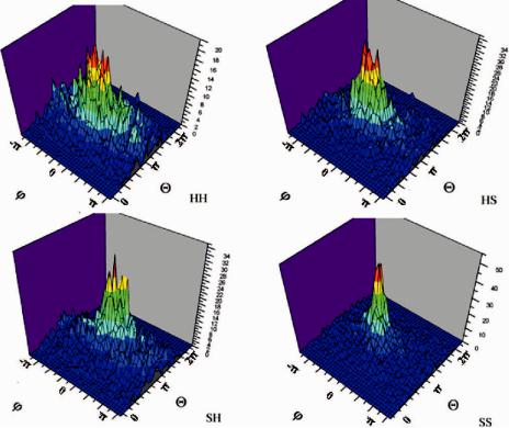
Fig. 11.16 Geometry of two consecutive secondary structures connected by a loop (Method II). The distributions of angles and for loop motifs of helix–helix (HH), helix–strand (HS), strand–helix (SH), and strand–strand (SS) are shown separately.
the ensemble of each accessible topology differs significantly due to the fact that, for some of the energetically unfavorable topology candidates, it was much harder to generate perturbed structures around the given skeleton that satisfied all of the criteria. A correlation is found between the number of perturbed structures and the average energy.
For the remaining seven proteins, three (2ezh, 1abv, and 1ngr) have their native topology recognized as the 2nd lowest in average energy (ranked as 2nd in the ninth column of Table 11.1). The topology of the lowest energy (1st) is very similar to the native topology (2nd) in all cases. Figure 11.17 schematically illustrates the three lowest energy topologies for protein 2ezh. The difference between the 1st and the native topology (2nd) was a swap of two helices that are very similar in length and nearby in space.
The native topologies of two other proteins, 2psr and 1l0i, were ranked 5th and 8th, respectively. Mismatches did happen between the assignment and skeleton for both cases: two helical regions were predicted as one in the assignment of 2psr, and