Computational Methods for Protein Structure Prediction & Modeling V1 - Xu Xu and Liang

(Krogh et al., 1994). Each node has a match state, insert state, and delete state. Each sequence uses a series of these states to traverse the model from start to end. Using a match state indicates that the sequence has a character in that column, while using a delete state indicates that the sequence does not. Insert states allow sequences to have additional characters between columns. In many ways, these models correspond to profiles. The primary advantage of these models over standard methods of sequence search is their ability to characterize an entire family of sequences.

7.2.5.4 Support Vector Machines

The SVM, first introduced by Vladimir Vapnik in 1992, is a linear learning machine based on recent advances in statistical theory (Vapnik, 1995, 1998) In other words, the main function of SVMs is to classify input patterns by first being trained on labeled data sets (supervised learning). SVMs have been shown to be a significant enhancement in function compared to other commonly used machine learning algorithms such as the perceptron algorithm (see Section 7.2.5.2, Neural Networks) and have been applied to many areas such as handwriting, face, voice, and object recognition and text characterization (for a comprehensive description of SVMs see Cristianini and Shawe-Taylor, 2000). With the turn of the millennium, SVMs were extensively applied to classification and pattern recognition problems in bioinformatics (for reviews see Byvatov and Schneider, 2003; Noble, 2004).

The power of SVMs lies in their use of nonlinear kernel (similarity) functions. When a linear algorithm such as the SVM uses a dot product, replacing it with a nonlinear kernel function allows it to operate in different space. Hence, the kernel functions used in SVMs implicitly map the input (training or test data) into high-dimensional feature spaces. In the high-dimensional feature spaces, linear classifications of the data are possible (each classifier is a separate dimension); they become nonlinear in following steps where they are transformed back to the original input space. As a result, although SVMs are linear learning machines regarding the high-dimensional feature spaces, in fact they act as nonlinear classifiers.

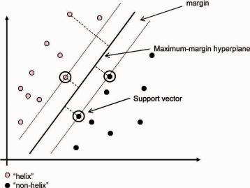
The key is to carefully design the kernel (similarity) criteria during training so as to best discriminate each class (for more information on kernels used in computational biology see Schoelkopf et al., 2004).Ultimately, the kernel function generates a maximum-margin hyperplane between two classes and resides somewhere in space (Fig. 7.6). For example, if we were training an SVM for helix prediction, given training examples labeled either “helix” or “nonhelix,” our kernel function would generate a maximum-margin hyperplane that would split the “helix” and “nonhelix” training examples so that the distance from the closest examples (the margin) to the hyperplane would be maximized (Fig. 7.6). If the hyperplane is not able to fully separate the “helix” and “nonhelix” examples, the SVM will choose a hyperplane that splits the examples as cleanly as possible, while still maximizing the distance to the nearest cleanly split examples. The parameters of the maximum-margin hyperplane are derived by solving a quadratic programming (QP) optimization problem. The examples closest to the hyperplane (decision boundary) are “support vectors,”

Fig. 7.6 SVM diagram illustrating an optimal separation of “helix” (red dots) and “nonhelix” (black dots) elements showing the position of the hyperplane.

while the ones far from it have no effect (Fig. 7.6). After training, any “unknown” input for which we want to decide whether it is helix or not is mapped into the high-dimensional space and the SVM decides whether it is “helix” or “nonhelix.” However, since secondary structure elements are usually classified in three states [helix (H), strand (E), and coil (C)], the actual recognition challenge is not binary (helix or nonhelix), but multiclass and therefore the prediction is still incomplete. The multiclass recognition problem is tackled differently across SVM prediction methods (Hua and Sun, 2001; Kim and Park, 2003; Ward et al., 2003; Guo et al., 2004; Hu et al., 2004), an example of which is described in Section 7.8.

7.2.6Consensus Secondary Structure Prediction

The majority of secondary structure prediction methods are trained using information from proteins of known 3D structure. In modern studies, training is performed on large data sets, thus avoiding overfitting, and the training data sets do not include any of the proteins used to assess the final version of the method (jack-knife testing). However, each method is trained on different sets of proteins and as a consequence this introduces a bias to the prediction performance, depending on the type of proteins used in the training set.

An early attempt to minimize these biasing effects was to combine predictions from various methods to produce a single consensus (Cuff et al., 1998; Cuff and Barton, 1999). The consensus was derived by majority voting, where the per-residue predicted states from each method were each given an equal “vote” and the consensus

kept the prediction that got the majority of the “votes.” The philosophy of deriving a consensus prediction is similar to that of having three clocks on a boat: if one clock shows the wrong time there are always the other two to check for consistency and since the probability that two out of three clocks will go wrong at the same time and in a similar way is very low, it is a safe assumption to go with the majority. During the same time, other strategies for consensus prediction were developed such as the combination of different NN outputs (Chandonia and Karplus, 1999; Cuff and Barton, 2000; King et al., 2000; Petersen et al., 2000); optimal method choice for the consensus scheme by linear regression statistics (Guermeur et al., 1999) and decision trees (Selbig et al., 1999); deriving a consensus from cascaded multiple secondary structure classifiers (Ouali and King, 2000); and expressing the consensus as a composite predicted secondary structure, where the variation in prediction is not resolved but used as extended information for the successive database searching steps for fold recognition (An and Friesner, 2002).

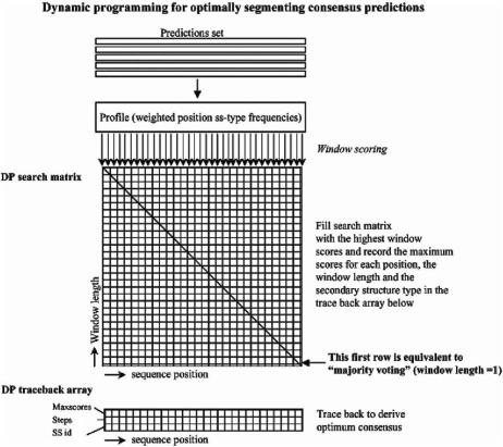
From these consensus-deriving strategies, the “majority voting” consensusderiving scheme has been employed in recent investigations using more state-of- the-art predictions methods and the results have consistently shown that a consensus prediction is better than any of the single predictions produced by the methods used for deriving the consensus (Albrecht et al., 2003; McGuffin and Jones, 2003; Ward et al., 2003). Recently, an extension to the “majority voting” dimensionality and segmentation capabilities was introduced by using dynamic programming (DP) to produce an optimally segmented consensus in an investigation of the effect of alignment gaps in secondary structure prediction (Simossis and Heringa, 2004a). The DP approach for generating a consensus has also very recently been applied to - barrel protein prediction (Bagos et al., 2005) and the generation of a consensus from multiple secondary structure prediction methods (Simossis and Heringa, 2005). In Fig. 7.7 we illustrate the relation between the “majority voting” and DP approaches. The original “majority voting” strategy is illustrated as a small part of the DP strategy, such that the window length of 1 (first row of the search matrix) represents the original “majority voting” and the remaining window lengths represent the added information used for the derivation of the consensus.

7.2.7Tertiary Structure Feedback for Secondary Structure Prediction

In the prediction techniques we have described up to now, predicting the secondary structure of a protein from its amino acid sequence has mainly involved using adjacent information. However, when a protein folds, the secondary structure elements that were initially formed can be influenced by the dynamics of formerly distant regions, which now have been brought closer due to the structural rearrangement in three-dimensional space (Blanco et al., 1994; Ramirez-Alvarado et al., 1997; Reymond et al., 1997). Although many initial conformations remain unchanged in the folded protein, there are regions that undergo transitions from one SSE type to

Fig. 7.7 The dynamic programming optimal segmentation strategy for deriving a consensus secondary structure prediction from multiple methods. The majority voting approach is limited to the first row of the search matrix, while the use of all possible segmentations of the information allows further optimization by dynamic programming.

another as a result of different types of interactions (Minor and Kim, 1996; Cregut et al., 1999; Luisi et al., 1999; Derreumaux, 2001; Macdonald and Johnson, 2001). As a result, even the best prediction methods make wrong predictions for these cases because the transition changes only happen as a result of tertiary structure interactions and have not yet occurred in the unfolded state.

Meiler and Baker (2003) used low-resolution tertiary structure models to feed back three-dimensional information to the predictions and successfully raised the quality of the predictions, particularly in -strands (Meiler and Baker, 2003). However, the applicability of the method is limited since it is only applicable to singledomain proteins and is not able to account for interdomain interactions.

In another approach, surface turns that change the overall direction of the chain (“U” turns) were predicted using multiple alignments and predicted secondary

structure propensities to improve the quality of the predictions (Hu et al., 1997; Kolinski et al., 1997).

7.3 Protein Supersecondary Structure Prediction

As a globular protein folds, different regions of the peptide backbone often come together (Wetlaufer, 1973; Unger and Moult, 1993). The compact combinations of two or more adjacent -strand and -helical structures, irrespective of the sequence similarity, form frequently recurring structural motifs that are known as supersecondary structures (Rao and Rossmann, 1973). Almost two-thirds of all residues in secondary structures are part of some type of supersecondary structure motif (Salem et al., 1999) and one-third of all known proteins can be classified into ten super folds, which are made up of different combinations between three basic supersecondary structures: the -hairpin, the -hairpin, and the - - motif (Salem et al., 1999).

The three basic types of supersecondary structure that are the most frequently observed include the - motifs ( -hairpins, -corners, and helix-turn-helix), themotif ( -hairpin), and the - - motif (two parallel -strands, separated by an -helix antiparallel to them, with two hairpins separating the three secondary structures). Other simple combinations of secondary structure types include the - -and - - motifs (Chothia, 1984). Some repetitions or combinations of the above simple supersecondary structures are also predominant in protein structures, such as the - - ( -meander), which is formed by two -hairpins sharing the middle strand. More elaborate supersecondary structure combination motifs include the Greek key (jellyroll) motif (Hutchinson and Thornton, 1993), the four-helix bundle (two - units connected by a loop), and the Rossman fold (effectively two - - units that each form one-half of an open twisted parallel -sheet). Although the majority of protein folds consist of several supersecondary structures, they can also be constituted by secondary structures in other contexts. An example of the latter is the globin fold, six of whose helices cannot be assigned to any of the aforementionedsupersecondary structures.

An interesting - motif is formed when a pair of -helices adopt a superhelical twist, resulting in a coiled-coil conformation. The usual left-handed coiled-coil interaction involves a repeated motif of seven helical residues (abcdefg), where the a and d positions are normally occupied by hydrophobic residues constituting the hydrophobic core of the helix–helix interface, while the other positions display a high likelihood to comprise polar residues. Another feature is that the heptad e and g positions are often charged and can form salt bridges.

An example of a more complex and higher-order supersecondary structure is the WD repeat (tryptophan-aspartate repeat), which is associated with a sequence motif approximately 31 amino acids long that encodes a structural repeat and usually ends with tryptophan-aspartic acid (WD). WD-repeat-containing proteins are thought to contain at least four copies of the WD repeat because all WD-repeat

proteins are speculated to form a circular -propeller structure. This is demonstrated by the crystal structure of the G protein -subunit, which is the only WD-repeat- containing structure available. It contains seven WD repeats, each of which folds into a small antiparallel -sheet. WD-repeat proteins have critical roles in many essential biological functions ranging from signal transduction, transcription regulation, to apoptosis, but are probably best known due to their association with several human diseases.

7.3.1Fundamentals of Supersecondary Structure Prediction

The identification of supersecondary structure motifs is largely, but not entirely, based on secondary structure prediction, as already discussed in Section 7.2. However, secondary structure information is a flat version of the protein structure, in contrast to supersecondary structure motifs that are recurring three-dimensional units that are formed when a protein folds. As a result, observing a pattern in secondary structure, e.g., strand–coil–strand, does not necessarily mean that it signifies a -hairpin supersecondary structure. On the contrary, such a basic secondary structure pattern could belong to a variety of different supersecondary structure motifs (Rost et al., 1997; de la Cruz and Thornton, 1999). Therefore, in order to extend from a collapsed secondary structure prediction to three-dimensional supersecondary structure prediction, a more detailed description of its properties is needed.

As described earlier, the secondary structure elements that make up supersecondary structure units are joined together by flexible regions that in the three-state classification of secondary structure are referred to as coil (C). Unlike the helix

(H) and strand (E) classes, coil adopts a wide range of conformations and is able to change the protein backbone into the different supersecondary structure motifs. As a result, identifying the properties of joining coil regions between helices and strands is the key to identifying a supersecondary structure motif type.

7.3.2Predicting Protein Supersecondary Structure

The methods that have been developed for the prediction of supersecondary structures have mainly employed machine learning techniques similar to those used in secondary structure prediction, namely, HMMs (Bystroff et al., 2000), NNs (Sun et al., 1997; Kuhn et al., 2004) and SVMs (Cai et al., 2003). In addition to these, some methods have also employed statistical regression techniques such as Monte Carlo-based simulations (Forcellino and Derreumaux, 2001) and a combination of secondary structure prediction and threading against known tertiary motifs (de la Cruz et al., 2002).

7.3.2.1 Neural Networks

Refer to Section 7.2.5.2 for an overview of NNs.

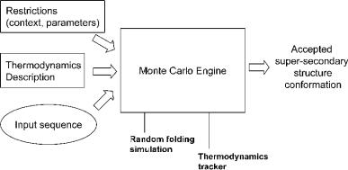
Fig. 7.8 A simplified representation of the Monte Carlo method for predicting supersecondary structure from sequence. This process is repeated enough times so that both the runtime and the accuracy are at acceptable levels.

7.3.2.2 Hidden Markov Models

Refer to Section 7.2.5.3 for an overview of HMMs.

7.3.2.3 Support Vector Machines

Refer to Section 7.2.5.4 for an overview of SVMs.

7.3.2.4 Monte Carlo Simulations

A Monte Carlo (MC) simulation is a stochastic technique, i.e. it uses random numbers and probability statistics to investigate problems (Fig. 7.8; for a comprehensive account see Frenkel and Smit, 2002). The invention of the MC method is often accredited to Stanislaw Ulam, a Polish mathematician who is primarily known for the design of the hydrogen bomb with Edward Teller in 1951. However, Ulam did not invent the concept of statistical sampling, but was the first to use computers to automate it. Together with John von Neumann and Nicholas Metropolis, he developed algorithms for computer implementations of the method, as well as means of transforming nonrandom problems into random forms that would facilitate their solution via statistical sampling. The method was first published in 1949 .()(Metropolis and Ulam, 1949). Nicholas Metropolis named the method after the casinos of Monte Carlo.

The strength and usefulness of MC methods is that they allow us to perform computations that would otherwise be impossible. For example, solving equations that describe the interactions between two atoms is fairly simple, but when attempting to solve the same equation for a fold or a whole protein (hundreds or thousands of atoms), the task is impossible. Basically, an MC simulation samples a large system in a number of random configurations. When selecting the number of random configurations, one way to minimize the standard error is to maximize the sample

size. However, due to the fact that this will be computationally expensive, a better solution is to restrict the variance of the random sample. As a result, depending on the restrictions applied to the MC simulation, configurations are accepted or rejected. Standard techniques of variance reduction include antithetic variates, control variates, importance sampling, and stratified sampling (see Frenkel and Smit, 2002).

In the case of protein structures, atoms are randomly moved in a predefined space so that the thermodynamics of the protein in a folded state are respected. The energies of these randomly folded proteins are calculated and according to a predefined selection criterion, they are kept as candidate structures or thrown away. The resulting set of candidate structures generated from this random sampling can be used to approximate the proteins folded state. The same principles apply to supersecondary structure prediction, where only the knowledge of the primary structure of short peptides is needed to sample a number of feasible conformations (Derreumaux, 2001).

7.4 Protein Disordered Region Detection

Disordered regions are regions of proteins or entire proteins, which lack a fixed tertiary structure, essentially because they are partially or fully unfolded. Disordered regions have been shown to be involved in a variety of functions, including DNA recognition, modulation of specificity/affinity of protein binding, molecular threading, activation by cleavage, and control of protein lifetimes. In a recent survey, Dunker et al. (2002) classified the functions of approximately 100 disordered regions into four broad categories: molecular recognition, molecular assembly/disassembly, protein modification, and entropic chains, the latter including flexible linkers, bristles, and springs (Dunker et al., 2002).

Although disordered regions lack a defined 3D structure in their native states, they frequently undergo disorder-to-order transitions upon binding to their partners. As it is known that the amino acid sequence determines a protein’s 3D structure, it is appropriate to assume that the amino acid sequence determines the lack of fixed 3D structure as well. Disordered proteins are found throughout the three kingdoms, but are predicted to be more common in eukaryotes than in archaea or eubacteria (Dunker et al., 2000). This would imply that intrinsic disorder is widespread but might be increasingly required for more complex protein functions.

Disordered proteins are gaining increased attention in the biological community (Wright and Dyson, 1999). Following the earlier work on protein folding by Ptitsyn (1994) on molten globule structures, native proteins have been divided in three folding states: ordered (fully folded), collapsed (molten globule-like), or extended (random coil-like). These three forms can occur in localized regions of proteins or comprise entire sequences. Protein function may arise from any of the three forms or from structural transitions between these forms resulting from changes in environmental conditions. The collapsed and extended forms correspond to intrinsic

disorder while the fully folded, ordered form is generally comprised of three secondary structure types: -helix, -sheet, and coil. However, since the collapsed (molten globule-like) state is known to have secondary structure, the presence or absence of secondary structure cannot be used to distinguish between ordered and disordered proteins. Another feature of disordered proteins or protein regions is that these are intrinsically dynamic and thus have relative coordinates and Ramachandran angles that vary significantly over time, while those in ordered proteins generally are comparatively invariant over time.

For proteins whose X-ray structures are known, the existence of disordered stretches can be identified directly by looking for amino acids that are missing from the electron density maps. A number of disordered regions in proteins have been directly characterized by NMR-based structure elucidation (Bracken, 2001; Dyson and Wright, 2002). Other sources of experimental evidence for disorder include a random coil-type circular dichroism spectrum and an extended hydrodynamic radius, while also limited, time-resolved proteolysis can provide useful information (Dunker et al., 2001).

As the accumulated experimental evidence of disordered regions is still limited and likely to cover only a small fraction of these regions existing in nature, alternative information-based prediction approaches have been developed. In accordance with the hypothesis that a protein’s structure and function are determined by its amino acid sequence, it is possible in principle to predict long stretches of 30 or more consecutive disordered residues from the primary structure. Distinguishing features for disordered regions include a higher average flexibility index value (Vihinen et al., 1994), a lower sequence complexity (Romero et al., 2001) as estimated by the popular NSEG method (Wootton and Federhen, 1996), a lower aromatic content (Xie et al., 1998), and different patterns regarding charge and hydrophobicity (Xie et al., 1998; Uversky et al., 2000). The state-of-the-art disorder prediction methods (Section 7.9.3) are thus generally based on the assumption that different types of disordered sequences are more similar to each other than to ordered sequences and vice versa, although protein regions in both the ordered and disordered class can display local variations in flexibility.

Young et al. (1999) successfully predicted regions likely to undergo structural change by using secondary structure prediction techniques. The authors examined protein regions for which secondary structure prediction methods gave equally strong preferences for two different states (Young et al., 1999). Such regions were then further processed combining simple statistics and expert rules. The final method was tested on 16 proteins known to undergo structural rearrangements, and on a number of other proteins. The authors reported no false positives, and identified most known disordered regions. The Young et al. method was further applied to the myosin family (Kirshenbaum et al., 1999), which led to the prediction of likely disordered regions that were previously unidentified, even though the tertiary structure of myosin was known.

In Section 7.9.3, a number of state-of-the-art methods are identified that have been developed especially for the prediction of protein disorder. These methods

include the PONDR suite (Obradovic et al., 2003), and the methods FoldIndex (Uversky et al., 2000), DISEMBL (Linding et al., 2003a), GLOBPLOT (Linding et al., 2003b), DISOPRED2 (Ward et al., 2004), PDISORDER (unpublished), and DISpro (Cheng et al., 2005). The highest prediction accuracies reported are currently beyond 90% (Cheng et al., 2005).

7.5 Internal Repeats Detection

7.5.1Genomic Repeats

An important characteristic of genomes, and particularly for those of eukaryotes, is the high frequency of internal sequence repeats. For example, the human genome is estimated to contain more than 50% of reiterated sequences (e.g., Heringa, 1998). One of the main evolutionary mechanisms for repeat duplication is recombination (Marcotte et al., 1999), which favors additional duplication after initial repeat copies have been made. In the case of tandem repeats, there is believed to be a pronounced correlation between copy number of repeats and further gene duplication (Heringa, 1994) due to gene slippage. Gene duplication can ease the selection pressure on an individual gene and thus lead to an accelerated divergence of the duplicated genes, thereby increasing the scope for evolution toward novel functions.

7.5.2Protein Repeats

Given widespread duplication and rearrangement of genomic DNA and subsequent gene fusion events, also at the protein level internal sequence repeats are abundant and found in numerous proteins. Gene duplication may enhance the expression of an associated protein or result in a pseudogene where less stringent selection of mutations can quickly lead to divergence resulting in an improved protein. An advantage of duplication followed by gene fusion at the protein level is that the protein resulting from the new single gene complex shows a more complex and often symmetrical architecture, conferring the advantages of multiple, regulated and spatially localized functionality. Many protein repeats comprise regular secondary structures and form multirepeat assemblies in three dimensions of diverse sizes and functions. In general, internal repetition affords a protein enhanced evolutionary prospects due to an enlargement of its available binding surface area. Constraints on sequence conservation appear to be relatively lax, for example due to binding functions ensuing from multiple, rather than, single repeats. Repeat proteins often fulfill important cellular roles, such as zinc-finger proteins that bind DNA, the-propeller domain of integrin -subunits implicated in cell–cell and cell– extracellular matrix interactions, or titin in muscle contraction, which consists of many repeated Ig and Fn3 domains. It is interesting in this regard that Marcotte et al. (1999) estimated that eukaryotic proteins are three times more likely to have internal repeats than prokaryotic proteins. The similarities found within sets of internal repeats can be 100% in the case of identical repeats, down to the level