

Computational Methods for Protein Structure Prediction & Modeling V1 - Xu Xu and Liang
.pdf5. Protein Structure Comparison and Classification |
167 |
As can be seen, there are gray areas in the SCOP database and scientists managing SCOP use their discretion in deciding these classifications.
CATH (Orengo et al., 1997) is created using the SSAP (Orengo and Taylor, 1996) program, and also tuned manually. Like SCOP, it is hierarchical and has four levels: class, architecture, topology, and homologous topology. Class is similar to SCOP’s class: proteins are categorized based on the types of SSEs they have. The architecture level classification of a protein is assigned manually based on the orientation of SSEs in 3D without considering their connectivity. At the topology level, SSE orientation and the connection between them are taken into account. At the lowest level, proteins are grouped into homologous topologies if there is sufficient evidence that they have an evolutionary relationship.
FSSP (Fold classification based on Structure-Structure alignment of Proteins) (Holm and Sander, 1996) is constructed using the DALI program (Holm and Sander, 1993). A representative set of all available protein structures is selected and all proteins in this representative set are aligned with each other. The resulting Z -scores are used to build a fold tree using an average linkage clustering algorithm. FSSP is fully automated.
Getz et al. (2002) assign SCOP and CATH classification to query proteins using FSSP; this assignment is based on the scores of the proteins in FSSP’s answer set for the query protein. They also found strong correlations between these classifications. The CATH topology of a protein can be identified from its SCOP fold with 93% accuracy, and the SCOP fold of a protein can be identified from its CATH topology with 82% accuracy.
5.5.2 Automated Classification
With an exponential growth in the number of newly discovered protein structures, manual databases have become harder to manage. Automated classification schemes that can produce classifications with a similar quality to the manual classifications are needed. Automated techniques are needed to find proteins that have similar structural features in a database that contains thousands of structures, especially with various distance metrics. Additionally, for recently discovered structures, the identification of the appropriate categories for their classification is crucial. It is not reasonable to expect every researcher to examine thousands of proteins to decide the classification of the new protein. Automated techniques are needed in this regard.
A number of schemes toward automated classification (Getz et al., 2002; Lindahl and Eloffson, 2000), fold recognition (Lundstrom et al., 2001; Portugaly and Linial, 2000), and structure prediction servers (Fischer, 2003; Kim et al., 2004) from protein sequences have been proposed. But, these schemes consider only the sequence information and ignore other sources of information that are available such as structure. An approach developed in Can et al. (2004) uses sequence and structure information simultaneously for the automated classification of proteins. This is discussed in detail next.
168 |
Orhan C¸ amo˘glu and Ambuj K. Singh |
In the protein classification problem, there is an existing classification scheme such as SCOP, and there is a set of new proteins that has to be classified based on the implicit rules and conventions of the existing classification. A classification algorithm simplifies the update of databases such as SCOP that have to accommodate many new proteins periodically. The main questions that need to be answered during classification are:
Does the query protein belong to an existing category (family/superfamily/fold), or does it need a new category to be defined?
If the query protein belongs to an existing category, what is its classification (label)?
The hierarchical nature of classification databases simplifies the classification problem. For example, if a protein belongs to a family, then its superfamily and fold are known. In the case of SCOP, the easiest classification level is family and the hardest one is fold. A hierarchical classifier can take advantage of this. The first attempt is to assign the protein to a family. If this is successful, then the other levels are already known. In case the protein does not belong to an existing family, a superfamily level classification is attempted. If the protein does not belong to an existing superfamily, a fold level classification is attempted.
5.5.3Building a Classifier from a Comparison Tool
Given a protein comparison tool (sequence or structure), a classifier can be designed by comparing a given query with all proteins of known classification. Similarity scores obtained thus provide a measure of proximity of the query protein to the categories defined in the classification. After sorting these scores, the first classification question (does the query belong to an existing category?) can be answered as follows. If none of the categories show a similarity greater than some predefined cutoff, the query protein is classified as not belonging to an existing category. This cutoff can be determined by investigating the score distribution of each tool.
A 1-Nearest-Neighbor (1NN) classification can be used for the second classification problem (what is the category of the query protein?). The query protein is assigned to the category of the protein that is found to be most similar, i.e., gets the highest score, using the comparison tool.
In Can et al. (2004), five component classifiers were defined using two sequence and three structure comparison tools. The first sequence tool uses the Hidden Markov Model (HMM) library from the SUPERFAMILY database (Gough, 2002). This library is manually curated to classify proteins at the SCOP superfamily level. The models in the SUPERFAMILY database can be searched using HMM-based search tools such as HMMER (Eddy, 1998) and SAM (Hughey and Krogh, 1995). These tools assign a similarity score to a protein sequence according to its match with a model. This classifier is referred to as HMMER.
The second sequence comparison tool is PSI-Blast (Altschul and Koonin, 1998). PSI-Blast is an improved version of Blast that works in iterations. In the
5. Protein Structure Comparison and Classification |
169 |
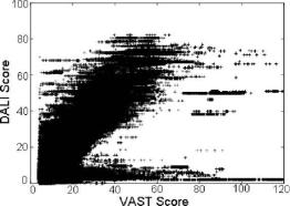
Fig. 5.14 Comparison of VAST and DALI scores for a set of proteins.
first iteration, Blast is run and a new scoring scheme is created based on the set of close neighbors. This process of searching and redefinition of score matrix can be repeated.
The structure comparison tools used were CE (Shindyalov and Bourne, 1998), VAST (Madej et al., 1995), and DALI (Holm and Sander, 1993). Each of these tools performs comparisons with a different technique. As a result, they provide a different view of structural relationships between proteins. For example, even though both VAST and DALI compare structures, they assign different scores to the same pair of proteins, as can be seen in Fig. 5.14. [In a similar study, Shindyalov and Bourne (2000) compared CE and DALI scores and showed that there were many proteins that were found similar by CE and dissimilar by DALI, and vice versa.] By exploiting these differences, one can achieve better performance with a combination of the tools.
Each sequenceand structure-comparison method described above assigns a score for a pair of proteins that indicates the statistical significance of the similarity between them. In particular, the z-scores reported by CE and DALI, p-values reported by VAST, and e-values (− log(e-value)) reported by HMMER and PSI-Blast are used as the similarity scores.
5.5.3.1 Performance of Component Classifiers
The individual performance (accuracy) of the tools when they are used as component classifiers was tested with a number of experiments. It was assumed that the classifications of all proteins in SCOP v1.59 (DS159) are known, and the goal of the component classifiers was to classify the new proteins introduced in SCOP v1.61 (QS161) into families, superfamilies, and folds. A hierarchical classification scheme is used (Camoglu et al., 2005). At the family level, all new proteins were queried. At the superfamily level, only proteins that do not have family-level similarities are queried. At the fold level, only proteins that do not have family/superfamily-level similarities are queried.

170 |
Orhan C¸ amo˘glu and Ambuj K. Singh |
At the family level, the sequence tools outperform the structure tools by achieving 94.5 and 92.6% accuracy. The highest success rate of the structure tools is only 89% by VAST. For 83% of the query proteins, all five tools make correct decisions (as to whether the query protein belongs to an existing category), for 4.1% of the queries four tools, for 1.9% of the queries three tools, for 6.9% of the queries two tools, and for 2.7% of the queries only one tool makes the correct decision. An interesting point here is that for 98.2% of the proteins, at least one tool is successful. So, it is theoretically possible to classify up to 98.2% of these proteins correctly by combining the results of the individual tools.
At the superfamily level, the performance of the structure tools improves relative to the sequence tools, as expected. However, the overall performance of the tools drops significantly compared to the family level. This is expected since classification at the superfamily level is harder. HMMER has one of the best performances with a 79.1% accuracy; this is no surprise considering that HMMER is manually tuned for superfamily classifications. Among the structure tools, VAST has the best performance with a 78.6% success rate. PSI-Blast performs poorly with a success rate of only 66.1%. Only 44.7% of the queries can be classified correctly by all five tools. For 4% of the queries, none of them is successful. This again raises the possibility of achieving better accuracy through a combination of the tools. These results are depicted in Fig. 5.15.
Structure tools outperform sequence tools at the fold level. VAST has the best performance with an 85% success rate. PSI-Blast has the worst performance with
Fig. 5.15 Performance of individual classifiers on recognizing the members of existing superfamilies, and assigning categories to them for the new proteins in SCOP v.1.61. The first set of bars represents the performance for recognition of existing members and the second set represents the performance for the assignment of categories.
5. Protein Structure Comparison and Classification |
171 |
a 60.7% success rate. For only 30.9% of the queries, all five tools are successful (Camoglu et al., 2005).
Once a tool has marked a new protein as a member of an existing category, the classification of the query protein is complete, i.e., the query protein is assigned to the same category as its nearest neighbor. The next question is to judge the accuracy of this assignment, i.e., whether the assigned category is the correct one. The accuracies of the tools are high at the family level. All except DALI have success rates above 90%. HMMER has the best performance with 94.8% accuracy and is followed by PSI-Blast with 92.3% accuracy. For 76.5% of the queries, all five tools are able to assign the correct family label. For only 2.1% of the queries, none of them is successful. The superfamily results can be seen in Fig. 5.15. At the fold level, all tools seem to perform poorly. At the fold level, PSI-Blast is not able to make even one correct fold assignment, whereas VAST assigns correct folds to 54% of the queries. For 35.1% of the queries, none of the tools is able to assign the correct fold label.
5.5.4 Automated Classification Using Ensemble Classifier
As evident from the earlier experiments, an ensemble classifier can potentially obtain higher classification accuracy than any single component classifier. There are many studies in the area of machine learning and pattern recognition that address the intelligent design of ensemble classifiers (Duda et al., 2001; Meir and Ratsch, 2003; Schapire and Singer, 1999). These include both competitive models (e.g., bagging and binning) and collaborative models (e.g., boosting).
Camoglu et al. (2005) employ a hierarchical decision tree to answer the question whether the query protein belongs to an existing category. To combine different tools, their results need to be normalized to a consistent scale. This is achieved by dividing the scores into bins. A bin is a tool-neutral accuracy extent, e.g., 90–100%, 80–100%, instead of a tool-specific similarity score. Bins for each tool are manually crafted to achieve maximum performance. All proteins’ 1NN scores are obtained and sorted. Bin boundaries are placed on this sorted list and accuracy is computed for each bin. For example, if bin i is labeled with an accuracy of x%, then the predicted accuracy of all proteins whose scores fall in the bin is x%.
After the bins for each tool are constructed, a decision tree is created. At each level of this tree, a combination of tools is run and depending on their decisions, query proteins are classified as a member of an existing category or new. The decision tree for the family level is presented in Fig. 5.16. As can be seen, at the first level of the decision tree, PSI-Blast and HMMER are run to classify the query protein. Each tool reports a confidence for their classification decision and these decisions and confidences are merged (Can et al., 2004). If the confidence of the consensus decision is greater than 95%, the query protein is classified as a member of an existing family. If the confidence is lower than 60%, it is classified as a member of a new family. If the confidence is between 60 and 95%, then tools at this level cannot make a confident decision, and the next level of the tree is used. At the next level, all of the structure tools are run for a consensus decision. There are again two thresholds,

172 Orhan C¸ amo˘glu and Ambuj K. Singh
|
Comparison Tool |
|
|
|
|
HMM+Blast |
|
|
|
<60% |
else |
|
>95% |
existing |
new family |
|
|
||
|
|
family |
||
|
|
|
|
|
|
CE + Vast + |
|
|
|
|
Dali |
|
|
|
<70% |
else |
>85% |
existing |
|
new family |
|
|
||
|
|
|
family |
|
|
HMM+Blast |
|
|
|
<85% |
|
>85% |
|
|
new family |
existing |
|
|
|
family |
|
|
||
|
|
|
|
|
Fig. 5.16 The decision tree for recognizing if a query protein belongs to an existing family.
85 and 70%. At the last level, there is only one threshold, 80%. If the confidence is greater than this threshold, the query protein is classified as a member of an existing family, else it is classified as a member of a new family.
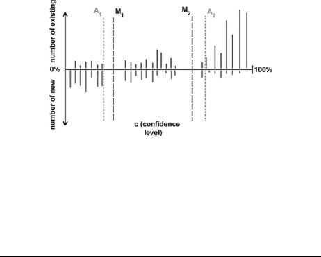
There are two components of a decision tree: (1) the combination of tools at each level and (2) the thresholds at each level. The first issue is addressed by using the domain knowledge of the classification schemes and the classification results for component classifiers (e.g., Fig. 5.15). For example, at the family level, it is known that sequence tools have priority, and at the superfamily level and fold levels, structure tools are more important. The problem of finding the right thresholds requires more care. The thresholds can be automatically determined by examining different choices and finding values that maximize accuracy for the training data. But, this approach tends to overfit. Thus, the distributions are manually analyzed and thresholds set after this analysis. An example of such an analysis is depicted in Fig. 5.17. Although placing the cutoff at point A2 is more suitable for the training data, it is clear that there is a natural separation at point M2. If A2 is used as the threshold, it overfits the data and the eventual performance suffers. The determined thresholds for superfamily and fold level classifications are shown in Table 5.1.
5.5.5Experimental Analysis
To validate that the consensus classifier indeed improves the classification performance, the standard validation technique in pattern recognition is applied (Duda et al., 2001). Two data sets are used: a training set and a test set. Ensemble classifier
5. Protein Structure Comparison and Classification |
173 |
Fig. 5.17 An example histogram of the confidence levels for the training data. A1 and A2 are the thresholds found by the automated greedy approach. M1 and M2 are the manual thresholds. It is seen that A1 and A2 overfit the data, whereas M1 and M2 do not.
Table 5.1 Heuristic decision tree rules for recognition of members of existing superfamilies and folds. At each level, a combination of tools is run and the probability of being a member of an existing category is assigned to each protein. The proteins that have probabilities higher than the indicated range are assigned to the predicted category, the ones within the range are passed to the next step, and those below the range are deemed new. For the last level, only a single threshold exists.
|
Level 1 |
Range |
Level 2 |
Range |
Level 3 |
Threshold |
|
|
|
|
|
|
|
Superfamily |
VAST |
45%:93% |
HMMER |
40%:75% |
CE+DALI |
55% |
Fold |
VAST |
50%:85% |
CE |
80%:90% |
DALI |
60% |
|
|
|
|
|
|
|
is trained with proteins introduced in SCOP 1.61 using the classifications of proteins in SCOP 1.59, and it is validated on proteins introduced in SCOP 1.63 using the classifications of proteins in SCOP 1.61. Automated ensemble classifier performed well on assigning proteins to their correct classifications by achieving 98% success for family assignments, 83% success for superfamily assignments, and 61% success for fold assignments. The performance of each tool and the ensemble classifier for superfamily classification (training and evaluation phases) is shown in Table 5.2. The benefits of an ensemble classifier are obvious. Complete results appear in Camoglu et al. (2005).
5.6 Concluding Remarks
A number of algorithms for protein comparison were presented in this chapter. Besides a survey of the current state of the art of techniques for problems in structure analysis such as pairwise alignment, multiple alignment, and motif discovery,

174 |
Orhan C¸ amo˘glu and Ambuj K. Singh |
Table 5.2 Performance of individual tools and ensemble classifier on training and test data sets. The performance is measured for two cases: Existing (ability to recognize the proteins from the existing classifications) and Assignment (ability to assign correct classifications)
|
|
|
|
Existing |
|
Assignment |
|
|
|
|
|
|
|
|
|
|
|
Training |
Evaluation |
Training |
Evaluation |
||
|
|
|
|
|
|
||
Superfamily |
HMMER |
78.63 |
79.29 |
68.9 |
39.18 |
||
|
CE |
71.77 |
38.03 |
81.1 |
43.81 |
||
|
VAST |
78.63 |
66.67 |
81.71 |
55.67 |
||
|
DALI |
77.42 |
75.24 |
80.49 |
74.74 |
||
|
PSI-Blast |
66.13 |
31.39 |
11.59 |
24.23 |
||
|
Ensemble |
80.65 |
83.82 |
93.29 |
82.99 |
||
|
|
|
|
|
|
|
|
techniques that scale to large data sets were discussed in depth. In this vein, an approach based on index structures was presented for pairwise protein structure comparison. In this technique, SSE-based features were extracted from database proteins and inserted into an index structure. Given a query protein, its features were also extracted and compared using the index. A graph-based approach was used to extend and evaluate the matches. Embedding this algorithm into well-known pairwise structure analysis algorithms led to significant speed-ups. As data sets such as the PDB grow in size, scalability of structure comparison algorithms will be an important factor.
Classification of proteins was also presented. A number of existing classification techniques based on protein structure were discussed. A technique for automated classification of proteins was investigated in depth. The approach used a number of sequence and comparison tools and combined them in a decision tree to increase the classification accuracy. The use of multiple data sources is an increasingly useful criterion in biological analysis. Some aspects of such an approach were presented in the use of multiple sequence and structure comparison tools for protein classification.
Comparing protein structures quantitatively poses a number of challenges: defining the appropriate notion of similarity, developing new algorithms based on these notions of similarity that can scale to an exponentially increasing number of structures, and understanding the significance of a score. The substantial amount of research in this area is a reflection of the current challenges and activity in this area. Other opportunities for future research include: flexible models for alignment, simultaneous use of sequence and structure in pairwise and multiple alignment, and evolutionary characterization of structures and protein–protein interactions.
5.7 References and Resources
5.7.1Definitions
Protein structure alignment: one-to-one mapping between the residues of two protein structures.

5. Protein Structure Comparison and Classification |
175 |
Root-mean-square distance: the root-mean-square distance (RMSD) between two proteins A and B under a correspondence R of size k and a transformation f is defined as
RMSD(A,B, R, f ) |
|
|
|
|
i=1 dist (ki |
i |
|
|
= |
|
|
|
k |
2 a |
, f (R(a ))) |
|
|
|
|
|
|
||
Distance matrix: a two-dimensional matrix where each entry Mi j stores the Euclidean distance between the ith and jth residues of a protein.
Structural motif: a substructure that is common in the structures of a set of proteins.
Multiple structure alignment: the alignment of a set of related proteins that results in a consensus structure which has the minimum RMSD sum to the protein structures in the set.
Feature vector: a vector composed of numerical values that summarizes the properties of an object.
Index structure: a data structure that organizes a set of objects and supports efficient retrieval.
5.7.2 |
Resources |
|
|
|
|
|
|
Name |
Description |
Link |
|
|
|
|
|
CATH |
Classification |
http://cathwww.biochem.ucl.ac.uk/latest/ |
|
CE |
Pairwise & multiple |
http://cl.sdsc.edu/ |
|
|
alignment |
|
|
DALI |
Pairwise alignment |
http://www.ebi.ac.uk/dali/ |
|
FSSP |
Classification |
http://ekhidna.biocenter.helsinki.fi/dali/start |
|
MASS |
Multiple alignment |
http://bioinfo3d.cs.tau.ac.il MASS/ |
|
MultiProt |
Multiple alignment |
http://bioinfo3d.cs.tau.ac.il/MultiProt/ |
|
PDB |
Structure repository |
http://www.rcsb.org/pdb/Welcome.do |
|
ProtDex |
Database search |
http://xena1.ddns.comp.nus.edu.sg/genesis/PD2˜ |
.htm |
PSI |
Database search |
http://bioserver.cs.ucsb.edu/proteinstructuresimilarity.php |
|
SCOP |
Classification |
http://scop.mrc-lmb.cam.ac.uk/scop/ |
|
SSAP |
Pairwise alignment |
http://www.cathdb.info/cgi-bin/cath/GetSsapRasmol.pl |
|
Trilogy |
Motif finding |
http://theory.lcs.mit.edu/trilogy/ |
|
URMS |
Pairwise alignment |
http://cbsusrv01.tc.cornell.edu/urms/ |
|
VAST |
Pairwise alignment |
http://www.ncbi.nih.gov/Structure/VAST/vastsearch.html |
|
|
|
|
|
5.8 Further Reading
For readers interested in pairwise protein structure comparison, we recommend “Protein structure comparison by alignment of distance matrices” by Holm and Sander (1993), “Approximate protein structural alignment in polynomial time” by
176 |
Orhan C¸ amo˘glu and Ambuj K. Singh |
Kolodny and Linial (2004), and “Sensitivity and selectivity in protein structure comparison” by Sierk and Pearson (2004). For more information on motif detection and multiple structure alignment, we recommend “Discovery of sequence–structure patterns across diverse proteins” by Bradley et al. (2002) and “MASS: multiple structural alignment by secondary structures” by Dror et al. (2003). More information about database searches can be found in “Index-based similarity search for protein structure databases” by Camoglu et al. (2004) and “Rapid 3d protein structure database searching using information retrieval techniques” by Aung and Tan (2004). For further discussion about the comparison of classification databases and automated classification techniques, we recommend “Automated assignment of SCOP and CATH protein structure classifications from FSSP scores” by Getz et al. (2002) and “Decision tree based information integration for automated protein classification” by Camoglu et al. (2005).
Acknowledgment
This work was supported in part by NSF grants DBI-0213903 and EF-0331697.
References
Alexandrov, N., and D. Fischer. 1996. Analysis of topological and nontopological structural similarities in the PDB: New examples from old structures. Proteins 25:354–365.
Altschul, S. F., and E. V. Koonin. 1998. Iterated profile searches with PSI-BLAST—a tool for discovery in protein databases. Trends Biochem Sci. 23:444–447.
Arun, K., T. Huang, and S. Blostein. 1987. Least-squares fitting of two 3-D point sets. IEEE Trans. Pattern Anal. Mach. Intell. 9:698–700.
Aung, Z., and K.-L. Tan. 2004. Rapid 3d protein structure database searching using information retrieval techniques. Bioinformatics 20:1045–1052.
Beckmann, N., H.-P. Kriegel, R. Schneider, and B. Seeger. 1990. The R*-tree: An efficient and robust access method for points and rectangles. In SIGMOD, pp. 322–331, Atlantic City, NJ.
Berman, H. M., J. Westbrook, Z. Feng, G. Gilliland, T. N. Bhat, H. Weissig, I. N. Shindyalov, and P. E. Bourne. 2000. The Protein Data Bank. Nucleic Acids Res. 28:235–242.
Binkowski, T. A., B. DasGupta, and J. Liang. 2004. Order independent structural alignment of circularly permuted proteins. In IEEE EMBS, July.
Bradley, P., P. S. Kim, and B. Berger. 2002. TRILOGY: Discovery of sequence– structure patterns across diverse proteins. Proc. Natl. Acad. Sci. USA 99:8500– 8503.
Brown, N., C. Orengo, and W. Taylor. 1996. A protein structure comparison methodology. Comput. Chem. 20:359–380.