

Computational Methods for Protein Structure Prediction & Modeling V1 - Xu Xu and Liang
.pdf1. A Historical Perspective and Overview |
43 |
Wriggers, W., Milligan, R. A., Schulten, K., and McCammon, J. A. 1998. Selforganizing neural networks bridge the biomolecular resolution gap. J. Mol. Biol. 284:1247–1254.
Xu, D., Baburaj, K., Peterson, C. B., and Xu, Y. 2001. Model for the threedimensional structure of vitronectin: Predictions for the multi-domain protein from threading and docking. Proteins 44:312–320.
Xu, J., Li, M., Kim, D., and Xu, Y. 2003. RAPTOR: Optimal protein threading by linear programming. J. Bioinform. Comput. Biol. 1:95–117.
Xu, Y., and Xu, D. 2000. Protein threading using PROSPECT: Design and evaluation. Proteins 40:343–354.
Ye, Y., Li, Z., and Godzik, A. 2006. Modeling and analyzing three-dimensional structures of human disease proteins. Pac. Symp. Biocomput. (Maui).
Yip, Y. L., Scheib, H., Diemand, A. V., Gattiker, A., Famiglietti, L. M., Gasteiger, E., and Bairoch, A. 2004. The Swiss-Prot variant page and the ModSNP database: A resource for sequence and structure information on human protein variants. Hum. Mutat. 23:464–470.
Yona, G., and Levitt, M. 2002. Within the twilight zone: A sensitive profile–profile comparison tool based on information theory. J. Mol. Biol. 315:1257–1275.
Yuan, Z., Mattick, J. S., and Teasdale, R. D. 2004. SVMtm: Support vector machines to predict transmembrane segments. J. Comp. Chem. 25:632–636.
Zhai, Y., and Saier, M. H. J. R. 2002. The -barrel finder (BBF) program, allowing identification of outer membrane -barrel proteins encoded within prokaryotic genomes. Protein Sci. 11:2196–2207.
Zhang, Y., and Skolnick, J. 2004. Automated structure prediction of weakly homologous proteins on a genomic scale. Proc. Natl. Acad. Sci. USA 101:7594–7599.
Zheng, Q., and Kyle, D. J. 1996. Accuracy and reliability of the scaling-relaxation method for loop closure: An evaluation based on extensive and multiple copy conformational samplings. Proteins 24:209–217.
Zhou, H., and Zhou, Y. 2005. Fold recognition by combining sequence profiles derived from evolution and from depth-dependent structural alignment of fragments. Proteins 58:321–328.
2 Empirical Force Fields
Alexander D. MacKerell, Jr.
Protein structure and dynamics and, therefore, their biological functions are dictated by a collection of forces that vary from those associated with covalent linkages, such as bonds, to long-range through space forces, such as electrostatic or coulombic interactions. Accordingly, to be able to apply theoretical approaches to understand the behavior of proteins, it is necessary to be able to accurately predict the change in energy of a protein as a function of the change in conformation. Importantly, such predictions must include contributions from the environment in which the protein is immersed. While quantum-mechanical (QM) methods are attractive in their ability to model complex chemical phenomena at the level of electronic structure, such methods are typically inappropriate for proteins due to the large size of these macromolecules as well as the need to treat their environment in an explicit fashion. Rather, molecular mechanics (MM), which rely on potential energy functions or empirical force fields, afford the computational speed to allow for calculations on proteins along with their environment.
2.1 Potential Energy Functions
The computational speed associated with molecular mechanics is based on the simplicity of the mathematical models used in the potential energy function to relate the structure of the system to its energy. This simplicity is based on the smallest particles in the model typically being atoms, which are treated as point masses centered on the nucleus of each atom in the molecules comprising the system under study. The potential energy function therefore describes the interactions between the atoms in the system.
An example of the potential energy function used in the additive CHARMM force fields (Brooks et al., 1983; MacKerell et al., 1998b) is shown in Eq. (2.1); similar energy functions are used in the common macromolecular force fields for proteins including OPLS/AA (Jorgensen and Tirado-Rives, 1988), AMBER (Cornell
45
46 |
Alexander D. MacKerell, Jr. |
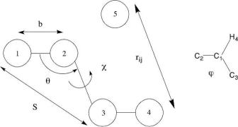
Fig. 2.1 Schematic diagram of the terms used to describe the energy as a function of the conformation in the potential energy function. The bond length between two covalently attached atoms 1 and 2 is b, is the valence angle between atoms 1, 2, and 3, is the dihedral angle involving atoms 1, 2, 3, and 4, S is the Urey-Bradley distance between atoms 1 and 3, and rij is the through space distance between atoms 1 and 4. The inset shows an example of an improper dihedral, , which is defined as the dihedral C1–C2–C3–H4.
et al., 1995), and GROMOS (van Gunsteren, 1987).
U (R) = |
|
|
|
|
|
|
|
|
|
|
||
Kb(b − b0)2 + K ( − 0)2 + KUB(S − S0)2 |
||||||||||||
|
bounds |
|
|
angle |
|
|
|
UB |
|
|
||
|
|
K (1 + cos(n − )) + |
|
Kimp( − 0)2 (2.1) |
||||||||
|
+ |
|
|
|||||||||
|
dihedrals |
|
|
|
|
|
|
impropers |
|
|
|
|
|
|
|
|
|
12 |
|
Rmin,ij |
|
6 |
qi q j |
|
|
|
|
|
|
|||||||||
|
+ nonbound εij |
|
Rmin,ij |
|
|
− 2 |
|
+ |
||||
|
rij |
|
rij |
|
4 erij |
|||||||
Equation (2.1), where the potential energy, U , is calculated as a function of the
atomic positions, R, includes terms for the internal (i.e., bonded) and external (i.e., interaction or nonbond) contributions. Internal terms include the bonds, valence angles, Urey-Bradley, dihedral or torsion angles, and improper dihedral terms while the external terms include the van der Waals (vdW) interations, treated via the Lennard-Jones (LJ) 6–12 term and the electrostatic interactions. In Eq. (2.1), terms describing the geometry of the molecule include the bond length, b, the valence angle,, the distance between atoms separated by two covalent bonds (Urey-Bradley term, 1,3 distance), S, the dihedral or torsion angle, , the improper angle, , and the distance between atoms i and j, rij. The schematic diagram in Fig. 2.1 illustrates the terms included in Eq. (2.1).
In order for the potential energy function to represent different types of, for example, bonds (e.g., C–C single versus double bonds) or atom types, parameters are used for each type of bond, angle, atom type, and so on in the molecules in the system. These parameters include the bond force constant and equilibrium distance, Kb and
2. Empirical Force Fields |
47 |
b0, respectively; the valence angle force constant and equilibrium angle, K , and 0; the Urey-Bradley force constant and equilibrium distance, KUB and S; the dihedral angle force constant, multiplicity, and phase angle, K , n, and ; and the improper force constant and equilibrium improper angle, K and 0. External parameters that describe the interactions between atoms i and j include the partial atomic charges, qi , and the LJ well-depth, εij, and minimum interaction radius, Rmin,ij, used to treat the vdW interactions. Typically, εi and Rmin,i are obtained for individual atom types and then combined to yield εij and Rmin,ij for the interacting atoms via combining rules. In CHARMM, εij values are obtained via the geometric mean (εij = sqrt(εi ε j ) and Rmin,ij via the arithmetic mean, Rmin,ij = (Rmin,i + Rmin, j )/2. The dielectric constant, e, is set to one in all calculations where solvent is considered explicitly (see below), corresponding to the permittivity of vacuum.
Essential for the modeling of proteins, as well as all biomolecules, is the proper treatment of hydrogen bonding. Earlier force fields included explicit terms for hydrogen bonds (Weiner and Kollman, 1981); however, it has been shown that the combination of the Lennard-Jones and coulombic interactions produces an accurate representation of both the distance and angle dependencies of hydrogen bonds (Reiher, 1985). This success has allowed for the omission of explicit terms to treat hydrogen bonding from the majority of empirical force fields. It should be noted that the LJ and electrostatic parameters are highly correlated, such that LJ parameters determined for a set of partial atomic charges will not be applicable to another set of charges. Moreover, the internal parameters are dependent on the external parameters. For example, the barrier to rotation about the C–O bond in ethanol includes contributions from the electrostatic and vdW interactions between the hydroxyl hydrogen and the rest of the molecule as well as contributions from the bond, angle, and dihedral terms. Thus, if the LJ parameters or charges are changed, the internal parameters will have to be reoptimized to produce the correct energy barrier. Finally, condensed phase properties obtained from empirical force field calculations contain contributions for the conformations of the molecules being studied as well as external interactions between those molecules, emphasizing the importance of accurate treatment of both internal and external portions of the force field for accurate condensed phase simulations.
Beyond the terms included in Eq. (2.1), additional terms may be included in a potential energy function; such extended energy functions are typically referred to as Class II force fields. Class II force fields can include higher order corrections for the bond and valence angle terms and/or cross terms between, for example, bonds and valence angles or valence angles and dihedrals (Lii and Allinger, 1991; Derreumaux and Vergoten, 1995; Halgren, 1996a; Sun, 1998; Ewig et al., 2001; Palmo et al., 2003). Other alternative terms include the use of a Morse function for bonds (Burkert and Allinger, 1982). This function allows for bond breaking to be included in an empirical force field. Another alternative is the use of a cosine-based valence angle term that is well behaved for near-linear valence angles (Mayo et al., 1990; Rapp´e et al., 1992). For the dihedral term a recent improvement that avoids singularities associated with derivatives of torsion angle cosines and allows for application of
48 |
Alexander D. MacKerell, Jr. |
any value of the phase has been presented (Blondel and Karplus, 1996) and, more recently, the introduction of a two-dimensional (2D) grid-based dihedral energy correction map (CMAP) (MacKerell et al., 2004a,b) that allows for any 2D dihedral surface (e.g., a QM , surface of the alanine dipeptide) to be reproduced nearly exactly by the force field (see below). These two terms are included in the recent version of the CHARMM force field for proteins. Typically inclusion of these terms in an energy function increases its accuracy in treating conformational energies, especially at geometries far from the minimum-energy or equilibrium values as well as yield improved treatment of vibrational spectra. However, it should be emphasized that Class I force fields [i.e., those based on Eq. (2.1)] can yield accuracies similar to the Class II force fields when the parameters are properly optimized. In general, Class I force fields, when applied to biomolecular simulations in the vicinity of room temperature, adequately treat the intramolecular distortions, including relative conformational energies associated with large structural changes.
The external portion of a potential energy function may also be extended beyond that in Eq. (2.1), including alternate forms of both the vdW interactions and the electrostatics. The three primary alternatives to the LJ 6–12 term included in Eq. (2.1) are designed to “soften” the repulsive wall associated with Pauli exclusion. For example, the Buckingham potential (Buckingham and Fowler, 1985) uses an exponential term to treat repulsion while a buffered 14–7 term is used in the MMFF force field (Halgren, 1996b). A simple alternative is to replace the r 12 repulsion with an r 9 term. All of these forms more accurately treat the repulsive wall as judged by high-level QM calculations (Halgren, 1992). However, as with the harmonic internal terms in Class I force fields, the LJ term appears to be adequate for biomolecular simulations at or near room temperature.
2.2 Implementation of Potential Energy Functions
As stated above, once an empirical force field is available, it may be used, in combination with the necessary software, to calculate the change of energy of a system as a function of coordinates. However, more useful is the combination of an empirical force field with numerical approaches allowing for sampling of relevant conformations via, e.g., a molecular dynamics (MD) simulation to be performed (Tuckerman and Martyna, 2000). Such approaches can be used to predict a variety of structural and thermodynamic properties, including free energies, via statistical mechanics (McQuarrie, 1976). Importantly, such approaches allow for comparisons with experimental thermodynamic data and the atomic details of interactions between molecules that dictate the thermodynamic properties can be obtained. Such atomic details are often difficult to access via experimental approaches, motivating the application of computational approaches.
Proper application of an empirical force field when performing MD simulations or other calculations on proteins is an essential consideration. Due to the central role of the external interactions in the energy function, it is important that all nonbond
2. Empirical Force Fields |
49 |
interactions between all atom–atom pairs be considered. The Ewald method can be used to treat the long-range electrostatic interactions for periodic systems (Ewald, 1921). Recent variations of the Ewald method that are computationally more tractable include the particle Mesh Ewald approach (Darden, 2001). Alternatively, reaction field methods can be used to simulate finite (e.g., spherical) systems (Beglov and Roux, 1994; Bishop et al., 1997; Im et al., 2001). Concerning the vdW or LJ interactions, the long-range contributions to this term beyond the atom–atom truncation distance (i.e., those beyond a distance where the atom–atom interactions are calculated explicitly) can be corrected for by assuming those contributions are homogeneous in nature (Allen and Tildesley, 1989; Lague et al., 2004).
The integrators that generate proper ensembles in MD simulations are another important consideration, as attaining the proper ensemble in an MD simulation is essential for direct comparison with experimental data (Tuckerman et al., 1992; Martyna et al., 1994; Feller et al., 1995; Barth and Schlick, 1998; Tuckerman and Martyna, 2000). Extensions of MD simulations have been developed that significantly increase the sampling of conformational space including locally enhanced sampling (Elber and Karplus, 1990; Hansmann, 1997; Simmerling et al., 1998) and replica-exchange or parallel tempering (Hansmann, 1997; Sugita and Okamoto, 1999; Nymeyer et al., 2004). It should be noted that the deterministic nature of MD simulations is typically lost when using such approaches, although the replicaexchange method can produce results that correspond to a proper ensemble. As always, the appropriate use of these different methods greatly facilitates investigations of molecular interactions via condensed phase simulations.
2.3 Treatment of Aqueous Solvation
Protein structure and function is greatly influenced by the condensed phase (i.e., aqueous) environment in which they exist. Accordingly, an empirical force field for proteins must treat the condensed phase environment in an accurate manner. Treatment of the protein environment may be performed using either explicit or implicit models. Explicit models, where the water, ions, and so on, are included explicitly in the simulation, are more microscopically accurate while implicit or continuum models can produce savings in computer time over explicit models and have the advantage of directly yielding free energies of solvation.
A number of explicit water models have been used in protein simulations including the TIP3P, TIP4P (Jorgensen et al., 1983), SPC, extended SPC/E (Berendsen et al., 1987) and F3C (Levitt et al., 1997) models. TIP3P is the most commonly used water model. Its three-point design (i.e., one oxygen and two hydrogen atoms) makes it computationally tractable and it yields the correct thermodynamic properties of water. Structurally the model treats the first and second solvation shells with reasonable accuracy. However, the second or tetrahedral peak in the O–O radial distribution is underestimated and the diffusion constant of the model is significantly larger than the corresponding experimental value (Feller et al., 1996). Another widely used
50 |
Alexander D. MacKerell, Jr. |
three-point model is SPC. This model uses an internal tetrahedral geometry (i.e., H–O–H angle = 109.47◦) leading to increased structure over TIP3P, as evidenced by a more-defined tetrahedral peak in the O–O radial distribution function. A variant of SPC, the SPC/E model, includes a correction for the polarization self-energy that yields improved structure and diffusion properties. However, this correction leads to an overestimation of the water potential energy in the bulk phase, which may perturb the energetic balance of solvent–solvent, solute–solvent, and solute–solute interactions. This problem must be considered when using this model in biomolecular simulations. TIP4P is a four-point water model that includes an additional particle along the H–O–H bisector. The additional particle overcomes many of the limitations listed above, although the computer demands of the model are higher. Recently, new water models have been presented (Mahoney and Jorgensen, 2000; Gl¨attli et al., 2003), although they have not seen wide use in biomolecular simulations.
Selection of the proper water model is important for a successful simulation. The most important consideration is the compatibility of the model with the biomolecular force field being used. Such compatibility is important due to most force fields being developed in conjunction with a specific water model (e.g., AMBER, OPLS and CHARMM with TIP3P, OPLS also with TIP4P, GROMOS with SPC, ENCAD with F3C), such that it is best to use a force field with its prescribed water model unless special solvent requirements are important.
Implicit solvation models treat the protein environment as a continuum, for example, by treating regions not “inside” the protein with the dielectric constant of water (Davis and McCammon, 1990; Honig, 1993). Such models offer significant computational savings while yielding reasonably accurate treatment of solvation. Accordingly, implicit models are useful when extensive sampling of conformational space is required, as in protein folding. However, these models can fail when highly specific water–biomolecule interactions have an important structural or energetic role. The most widely used implicit solvation models are Poisson-Boltzmann (PB) and generalized Born (GB) models. In the PB model, contributions from solvent polarization along with the asymmetric shapes of biological molecules are taken into account (Gilson and Honig, 1988), from which free energies of solvation may be determined. Advances in this approach have included the optimization of atomic radii to reproduce experimental free energies of solvation of model compounds representative of proteins (Nina et al., 1997; Banavali and Roux, 2002). GB approaches (Still et al., 1990) are an alternative to PB that also yield free energies of solvation while being less computationally expensive, thereby facilitating their use in MD simulations. Several GB models have been developed that yield free energies of solvation at a level of accuracy similar to PB methods (Schaefer and Karplus, 1996; Jayaram et al., 1998; Onufriev et al., 2000; Zhang et al., 2001; Lee et al., 2003). Both the PB and GB methods can be combined with free energy solvent accessibility (SA) terms that account for the hydrophobic effect (Qui et al., 1997; Gallicchio et al., 2003), referred to as PB/SA or GB/SA approaches. Recent developments based on the GB method involve an improved treatment of vdW dispersion contributions beyond the typical solvent accessibility related terms (Gallicchio and Levy, 2004). Other implicit
2. Empirical Force Fields |
51 |
models that have been used in biomolecular simulations include the Langevin Dipoles Model (Flori´an and Warshel, 1997) and the EEF1 model (Lazaridis and Karplus, 1999). More information on implicit solvating models can be obtained from a recent review by Feig and Brooks (Feig and Brooks, 2004).
The PB/SA and GB/SA methods can be used for postprocessing of trajectories from MD simulations to obtain free energies of solvation. In this approach an MD simulation of the biomolecule(s) is performed using an explicit solvent representation followed by estimation of the free energy of solvation using the solute coordinates from the simulation (i.e., biomolecule only with the solvent omitted) (Kollman et al., 2000). This allows for determination of the free energy of solvation of a biomolecule averaged over the length of a simulation, using structures obtained with an explicit solvent representation. This approach is particularly attractive for the calculation of free energies of binding of macromolecular complexes (Jayaram et al., 2002; Gohlke et al., 2003; Habtemariam et al., 2005). This type of approach also has great utility for the estimation of ligand–protein binding (Ferrara et al., 2004), at a computationally reasonable cost as required for testing of large numbers of drug candidates.
2.4 Empirical Force Field Optimization
The ability of a simple potential energy function such as that in Eq. (2.1) to accurately model the energies as a function of protein conformation is based on proper optimization of the parameters used in the energy function. Indeed, until the parameters are available, one does not truly have an empirical force field. And the quality of that empirical force field is judged by its ability to accurately reproduce the experimental regimen.
Parameter optimization is based on reproducing a set of target data, including information on small model compounds representative of proteins as well as on proteins themselves. Target data are ideally obtained from experiments, though a majority of the data are often obtained from QM calculations. QM calculations are readily applicable to most small molecules; however, limitations in QM level of theory, especially with respect to the treatment of dispersion interactions (Chalasinski and Szczesniak, 1994; Chen et al., 2002), require the use of experimental data when available (MacKerell, 2004).
Details on the optimization of internal parameters have been presented previously by a number or workers (Halgren, 1996c; Ewig et al., 2001; MacKerell, 2001; Wang and Kollman, 2001). Briefly, the equilibrium bond, valence angle, and Urey-Bradley parameters along with the dihedral multiplicity and phase are optimized to reproduce internal geometries of the model compounds. The target data are often QM data, although it has been shown that condensed phase effects can influence the internal geometry of a molecule, such that survey data from structures in the Cambridge Structural Database (CSD, http://www.ccdc.cam.ac.uk/) (Allen et al., 1979) may be considered the ideal. The value of such data for treatment of
52 |
Alexander D. MacKerell, Jr. |
the peptide bond has previously been discussed (MacKerell et al., 1998; MacKerell, 2004). Force constants for the bond, valence angle, Urey-Bradley, dihedral angle, and improper angles are optimized to reproduce vibrational spectra, including both the frequencies as well as the potential energy distribution (PED) (i.e., the contribution of internal degrees of freedom to the individual frequencies). Again the ideal data are obtained from condensed phase vibrational studies, although such data are typically limited making vibrational data from QM calculations the most commonly used. It should be emphasized that QM vibrational analysis allows for detailed assignment of the PED and, even when good experimental data are available, QM calculations are often advantageous to perform the assignments. When performing optimization of vibrational spectra, it should be noted that the low-frequency modes represent the largest structural distortions that occur in a molecule, such that their proper treatment is important for accurately treating the structural distortions that occur during MD simulations. Conformational energies from QM calculations, including barrier heights for rotations about dihedrals, are typically used for the final optimization of the dihedral angle parameters. In the CHARMM force fields the dihedral parameters are initially optimized based on vibrational data with only the parameters associated with dihedrals that involve all nonhydrogen atoms adjusted to reproduce potential energy surfaces. This final optimization is again important as the rotations about dihedrals represent the largest structural changes that occur in MD simulations of proteins. Recent work on lipids emphasizes the importance of proper treatment of the conformational energies (Klauda et al., 2005). In addition, empirical optimization of dihedral parameters to reproduce experimental distributions of conformers, such at the phi, psi angle distributions in proteins, have been shown to be important (MacKerell et al. 2004a,b). Those efforts have included optimization of the grid-based energy correction map discussed below.
Significant effort by a number of groups has gone into the determination of the electrostatic parameters; the partial atomic charges, qi . Of the methods currently in use, the most common methods for proteins are the supramolecular and QM electrostatic potential (ESP) approaches. Other variations include bond charge increments (Bush et al., 1999; Jakalian et al., 2000) and electronegativity equilization methods (Gilson et al., 2003), although these methods are typically applied to small, druglike molecules. An important consideration with the determination of partial atomic charges, related to the Coulombic treatment of electrostatics, is the omission of the explicit treatment of electronic polarizability. Due to this omission, it is necessary for static, partial atomic charges to reproduce the average polarization that occurs in the condensed phase environment. This is achieved by “enhancing” the charges of a molecule leading to an overestimation of the dipole moment as compared to the gas phase value. This is referred to as an implicitly polarized model. For example, many of the water models used in protein empirical force fields (e.g., TIP3P, TIP4P, SPC) have dipole moments in the vicinity of 2.2 debye (Jorgensen et al., 1983), versus the gas phase value of 1.85 debye. Inclusion of implicit polarizability allows for empirical force fields based on Eq. (2.1), which are often referred to as additive, to reproduce a variety of condensed phase properties (Rizzo and Jorgensen, 1999).
2. Empirical Force Fields |
53 |
These additive models have been extensively used for simulations of proteins, as well as other biological molecules; however, they are limited in that they do not reproduce the change in electrostatic interactions due to inductive effects associated with changes in the polarity of the environment.
The supramolecular approach for the determination of partial atomic charges is used in the OPLS (Jorgensen and Tirado-Rives, 1988; Jorgensen et al., 1996) and CHARMM (MacKerell et al., 1998b; Foloppe and MacKerell, 2000; Feller et al., 2002) force fields. This approach involves optimization of the charges to reproduce QM-determined minimum interaction energies and geometries of a model compound with individual water molecules or for model compound dimers. Typically, the HF/6-31G* level of theory was used for the QM calculations, due to its overestimation of dipole moments (Cieplak et al., 1995), leading to the implicitly polarizable model discussed above. An additional advantage of the supramolecular approach is that in the QM calculation, local polarization effects due to the charge induction caused by the two interacting molecules are included, facilitating determination of charge distributions appropriate for the condensed phase.
It should be noted that although it has recently been shown that QM methods can accurately reproduce gas phase experimental interaction energies for a range of model compound dimers (Kim and Friesner, 1997; Huang and MacKerell, 2002), it is important to maintain the QM level of theory that was historically used for a particular force field when extending that force field to novel molecules. This assures that the balance of the nonbond interactions between different molecules in the system being studied is maintained. Finally, when considering the transferability of charges obtained from the supramolecular approach, it should be noted that the charges are typically obtained for functional groups such that they may be directly transferred between molecules.
The other commonly applied approach for charge determination in empirical force fields is ESP charge fitting. This methodology is based on the adjustment of charges to reproduce a QM-determined ESP mapped onto a grid surrounding the model compound. ESP methods are widely used and a number of charge fitting methods based on this approach have been developed (Singh and Kollman, 1984; Chirlian and Francl, 1987; Merz, 1992; Bayly et al., 1993; Henchman and Essex, 1999). Application of ESP fitting approaches is hampered by difficulties in unambiguously fitting charges to an ESP (Francl et al., 1996) and charges on “buried” atoms (e.g., a carbon to which three or four nonhydrogen atoms are covalently bound) tend to be underdetermined, requiring the use of restraints during fitting (Bayly et al., 1993). The latter method is referred to as Restrained ESP (RESP). In addition, the QM ESP is typically determined via gas phase calculations, which may yield charges that are not consistent with the condensed phase. Recent developments are addressing this limitation (Laio et al., 2002). Another problem is that multiple conformations of flexible molecules must also be taken into account (Cieplak et al., 1995), although it should be noted that the last two problems are also present to varying extents in the supramolecular approach. For ESP fitting, the QM level of theory has historically been HF/6-31G*, as used in the AMBER force fields (Cornell et al., 1995), although