Computational Methods for Protein Structure Prediction & Modeling V1 - Xu Xu and Liang

where the weight coefficients are derived from database statistics. The objectives of optimization are often maximization of the energy gap between native protein and the average of decoys, or the energy gap between native and decoys with the lowest score, or the z-score of the native protein (Goldstein et al., 1992; Maiorov and Crippen, 1992; Thomas and Dill, 1996a; Koretke et al., 1996, 1998; Hao and Scheraga, 1996; Mirny and Shakhnovich, 1996; Vendruscolo and Domanyi, 1998; Tobi et al., 2000; Vendruscolo et al., 2000; Dima et al., 2000; Micheletti et al., 2001; Bastolla et al., 2001).

3.4.1 Geometric Nature of Discrimination

There is a natural geometric view of the inequality requirement for weighted linear sum potential functions. A useful observation is that each of the inequalities divides the space of Rd into two halves separated by a hyperplane (Fig. 3.4a). The hyperplane for Eq. 3.42 is defined by the normal vector (cN − cD ) and its distance b/||cN − cD || from the origin. The weight vector w must be located in the halfspace opposite the direction of the normal vector (cN − cD ). This half-space can be written as w · (cN − cD ) + b < 0. When there are many inequalities to be satisfied simultaneously, the intersection of the half-spaces forms a convex polyhedron (Edelsbrunner, 1987). If the weight vector is located in the polyhedron, all the inequalities are satisfied. Scoring functions with such weight vector w can discriminate the native protein sequence from the set of all decoys. This is illustrated in Fig. 3.4a for a two-dimensional toy example, where each straight line represents an inequality w · (cN − cD ) + b < 0 that the potential function must satisfy.

For each native protein i , there is one convex polyhedron Pi formed by the set of inequalities associated with its decoys. If a potential function can discriminate simultaneously n native proteins from a union of sets of sequence decoys, the weight vector w must be located in a smaller convex polyhedron P that is the intersection of the n convex polyhedra:

n

w P = Pi .

i =1

There is yet another geometric view of the same inequality requirements. If we now regard (cN − cD ) as a point in Rd , the relationship w · (cN − cD ) + b < 0 for all sequence decoys and native proteins requires that all points {cN − cD } are located on one side of a different hyperplane, which is defined by its normal vector w and its distance b/||w|| to the origin (Fig. 3.4b). We can show that such a hyperplane exists if the origin is not contained within the convex hull of the set of points {cN − cD } (see Appendix).

The second geometric view looks very different from the first view. However, the second view is dual and mathematically equivalent to the first geometric view. In the first view, a point cN − cD determined by the structure–decoy pair cN = (sN , aN ) and cD = (sN , aD ) corresponds to a hyperplane representing an inequality,

Fig. 3.4 Geometric views of the inequality requirement for protein scoring function. Here we use a two-dimensional toy example for illustration. (a). In the first geometric view, the space R2 of w = (w1, w2) is divided into two half-spaces by an inequality requirement, represented as a hyperplane w · (cN − cD ) + b < 0. The hyperplane, which is a line in R2, is defined by the normal vector (cN − cD ) and its distance b/||cN − cD || from the origin. In this figure, this distance is set to 1.0. The normal vector is represented by a short line segment whose direction points away from the straight line. A feasible weight vector w is located in the half-space opposite to the direction of the normal vector (cN − cD ). With the given set of inequalities represented by the lines, any weight vector w located in the shaped polygon can satisfy all inequality requirement and provides a linear scoring function that has perfect discrimination. (b) A second geometric view of the inequality requirement for linear protein scoring function. The space R2 of x = (x1, x2), where x ≡ (cN − cD ), is divided into two half-spaces by the hyperplane w · (cN − cD ) + b < 0. Here the hyperplane is defined by the normal vector w and its distance b/||w|| from the origin. The origin corresponds to the native protein. All points {cN − cD } are located on one side of the hyperplane away from the origin, therefore satisfying the inequality requirement. That is, a linear scoring function w such as the one represented by the straight line in this figure can have perfect discrimination. (c) In the second toy problem, a set of inequalities are represented by a set of straight lines according to the first geometric view. A subset of the inequalities require the weight vector w to be located in the shaded convex polygon on the left, but another subset of inequalities require w to be located in the dashed convex polygon on the top. Since these two polygons do not intersect, there is no weight vector w that can satisfy all inequality requirements. That is, no linear scoring function can classify these decoys from native protein. (d) According to the second geometric view, no hyperplane can separate all points {cN − cD } from the origin. But a nonlinear curve formed by a mixture of Gaussian kernels can have perfect separation of all vectors {cN − cD } from the origin: It has perfect discrimination.

and a solution weight vector w corresponds to a point located in the final convex polyhedron. In the second view, each structure–decoy pair is represented as a point cN − cD in Rd , and the solution weight vector w is represented by a hyperplane separating all the points C = {cN − cD } from the origin.

3.4.2 Optimized Linear Potential Functions

Several optimization methods have been applied to find the weight vector w of linear potential function. The Rosenblantt perceptron method works by iteratively updating an initial weight vector w0 (Vendruscolo and Domanyi, 1998; Micheletti et al., 2001). Starting with a random vector, e.g., w0 = 0, one tests each native protein and its decoy structure. Whenever the relationship w · (cN − cD ) + b < 0 is violated, one updates w by adding to it a scaled violating vector · (cN − cD ). The final weight vector is therefore a linear combination of protein and decoy count vectors:

Here N is the set of native proteins, and D is the set of decoys. The set of coefficients { N } { D } gives a dual form representation of the weight vector w, which is an expansion of the training examples including both native and decoy structures.

According to the first geometric view, if the final convex polyhedron P is nonempty, there can be an infinite number of choices of w, all with perfect discrimination. But how do we find a weight vector w that is optimal? This depends on the criterion for optimality. For example, one can choose the weight vector w that minimizes the variance of score gaps between decoys and natives:

as used in Tobi et al. (2000), or minimizing the Z -score of a large set of native proteins, or minimizing the Z -score of the native protein and an ensemble of decoys (Chiu and Goldstein, 1998; Mirny and Shakhnovich, 1996), or maximizing the ratio R between the width of the distribution of the score and the average score difference between the native state and the unfolded ones (Goldstein et al., 1992; Hao and Scheraga, 1999). A series of important works using perceptron learning and other optimization techniques (Friedrichs and Wolynes, 1989; Goldstein et al., 1992; Tobi et al., 2000; Vendruscolo and Domanyi, 1998; Dima et al., 2000) showed that effective linear sum potential functions can be obtained.

There is another optimality criterion according to the second geometric view (Hu et al., 2004). We can choose the hyperplane (w, b) that separates the set of points {cN − cD } with the largest distance to the origin. Intuitively, we want to characterize proteins with a region defined by the training set points {cN − cD }. It is desirable

to define this region such that a new unseen point drawn from the same protein distribution as {cN − cD } will have a high probability of falling within the defined region. Nonprotein points following a different distribution, which is assumed to be centered around the origin when no a priori information is available, will have a high probability of falling outside the defined region. In this case, we are more interested in modeling the region or support of the distribution of protein data, rather than estimating its density distribution function. For linear potential function, regions are half-spaces defined by hyperplanes, and the optimal hyperplane (w, b) is then the one with maximal distance to the origin. This is related to the novelty detection problem and single-class support vector machine studied in statistical learning theory (Vapnik and Chervonenkis, 1964, 1974; Scholkopf¨ and Smola, 2002). In our case, any nonprotein points will need to be detected as outliers from the protein distribution characterized by {cN − cD }. Among all linear functions derived from the same set of native proteins and decoys, an optimal weight vector w is likely to have the least amount of mislabelings. The optimal weight vector w can be found by solving the following quadratic programming problem:

The solution maximizes the distance b/||w|| of the plane (w, b) to the origin. We obtained the solution by solving the following support vector machine problem:

Minimize 12 w 2

subject to w · cN + d ≤ −1 (3.46) w · cD + d ≥ 1,

where d > 0. Note that a solution of Problem (3.46) satisfies the constraints in Inequalities (3.45), since subtracting the second inequality here from the first inequality in the constraint conditions of (3.46) will give us w · (cN − cD ) + 2 ≤ 0.

3.4.3Optimized Nonlinear Potential Functions

Optimized linear potential function can be obtained using the optimization strategy discussed above. However, it is possible that the weight vector w does not exist, i.e., the final convex polyhedron P = in=1 Pi may be an empty set. This occurs if a large number of native protein structures are to be simultaneously stabilized against a large number of decoy conformations, no such potential functions in the linear functional form can be found (Vendruscolo et al., 2000; Tobi et al., 2000).

According to our geometric pictures, there are two possible scenarios. First, for a specific native protein i , there may be severe restriction from some inequality constraints, which makes Pi an empty set. Some decoys are very difficult to discriminate due to perhaps deficiency in protein representation. In these cases, it is impossible to adjust the weight vector so the native protein has a lower score than the sequence decoy. Fig. 3.4c shows a set of inequalities represented by straight lines according

to the first geometric view. In this case, there is no weight vector that can satisfy all these inequality requirements. That is, no linear potential function can classify all decoys from native protein. According to the second geometric view (Fig. 3.4d), no hyperplane can separate all points (black and green) {cN − cD } from the origin, which corresponds to the native structures.

Second, even if a weight vector w can be found for each native protein, i.e., w is contained in a nonempty polyhedron, it is still possible that the intersection of n polyhedra is an empty set, i.e., no weight vector can be found that can discriminate all native proteins from the decoys simultaneously. Computationally, the question whether a solution weight vector w exists can be answered unambiguously in polynomial time (Karmarkar, 1984). If a large number (e.g., hundreds) of native protein structures are to be simultaneously stabilized against a large number of decoy conformations (e.g., tens of millions), no such potential functions can be found computationally (Vendruscolo et al., 2000; Tobi et al., 2000). A similar conclusion is drawn in a study on protein design, where it was found that no linear potential function can simultaneously discriminate a large number of native proteins from sequence decoys (Hu et al., 2004).

A fundamental reason for such failure is that the functional form of linear sum is too simplistic. It has been suggested that additional descriptors of protein structures such as higher order interactions (e.g., three-body or four-body contacts) should be incorporated in protein description (Betancourt and Thirumalai, 1999; Munson and Singh, 1997; Zheng et al., 1997). Functions with polynomial terms using up to 6 degrees of Chebyshev expansion have also been used to represent pairwise interactions in protein folding (Fain et al., 2002).

We now discuss an alternative approach. Let us still limit ourselves to pairwise contact interactions, although it can be naturally extended to include threeor fourbody interactions (Li and Liang, 2005b). We can introduce a nonlinear potential function analogous to the dual form of the linear function in Eq. (3.43), which takes the following form:

where D ≥ 0 and N ≥ 0 are parameters of the potential function to be determined, and cD = f (sN , aD ) from the set of decoys D = {(sN , aD )} is the contact vector of a sequence decoy D mounted on a native protein structure sN , and cN = f (sN , aN ) from the set of native training proteins N = {(sN , aN )} is the contact vector of a native sequence aN mounted on its native structure sN . In this study, all decoy sequences {aD } are taken from real proteins possessing different fold structures. The difference of this functional form from the linear function in Eq. (3.43) is that a kernel function K (x, y) replaces the linear term. A convenient kernel function K is

K (x, y) = e−||x− y||2 /2 2 for any vectors x and y N D,

where 2 is a constant. Intuitively, the surface of the potential function has smooth Gaussian hills of height D centered on the location cD of decoy protein D, and has

smooth Gaussian cones of depth N centered on the location cN of native structures N . Ideally, the value of the potential function will be −1 for contact vectors cN of native proteins, and will be +1 for contact vectors cD of decoys.

3.4.4Deriving Optimized Nonlinear Potential Functions

To obtain the nonlinear potential function, our goal is to find a set of parameters { D , N } such that H ( f (sN , aN )) has value close to −1 for native proteins, and the decoys have values close to +1. There are many different choices of { D , N }. We use an optimality criterion originally developed in statistical learning theory (Vapnik, 1995; Burges, 1998; Scholkopf¨ and Smola, 2002). First, we note that we

have implicitly mapped each structure and decoy from R210 through the kernel function of K (x, y) = e−||x− y||2 /2 2 to another space with dimensions as high as

tens of millions. Second, we then find the hyperplane of the largest margin distance separating proteins and decoys in the space transformed by the nonlinear kernel. That is, we search for a hyperplane with equal and maximal distance to the closest native proteins and the closest decoys in the transformed high dimensional space. Such a hyperplane can be found by obtaining the parameters { D } and { N } from solving the following Lagrange dual form of quadratic programming problem:

where C is a regularizing constant that limits the influence of each misclassified protein or decoy (Vapnik and Chervonenkis, 1964, 1974; Vapnik, 1995; Burges, 1998; Scholkopf¨ and Smola, 2002), and yi = −1 if i is a native protein, and yi = +1 if i is a decoy. These parameters lead to optimal discrimination of an unseen test set (Vapnik and Chervonenkis, 1964, 1974; Vapnik, 1995; Burges, 1998; Scholkopf¨ and Smola, 2002). When projected back to the space of R210, this hyperplane becomes a nonlinear surface. For the toy problem of Fig. 3.4, Fig. 3.4d shows that such a hyperplane becomes a nonlinear curve in R2 formed by a mixture of Gaussian kernels. It separates perfectly all vectors {cN − cD } (black and green) from the origin. That is, a nonlinear potential function can have perfect discrimination.

3.4.5Optimization Techniques

The techniques that have been used for optimizing potential function include perceptron learning, linear programming, gradient descent, statistical analysis, and support vector machine (Tobi et al., 2000; Vendruscolo et al., 2000; Xia and Levitt, 2000; Bastolla et al., 2000, 2001; Hu et al., 2004). These are standard techniques that can be found in optimization and machine learning literature. For example, there are excellent linear programming solvers based on simplex method, as implemented in CLP, GLPK, and LP SOLVE (Berkelaar, 2004), and based on interior point method as implemented in the BPMD (M´esz´aros, 1996), the HOPDM, and the PCX packages (Czyzyk

et al., 2004). We neglect the details of these techniques and point readers to the excellent treatises of Papadimitriou and Steiglitz (1998) and Vanderbei (1996).

3.5 Applications

Knowledge-based potential function has been widely used in the study of protein structure prediction, protein folding, and protein–protein interaction. In this section, we discuss briefly some of these applications. Additional details of applications of knowledge-based potential can be found in other chapters of this book.

3.5.1 Protein Structure Prediction

Protein structure prediction is an extraordinarily complex task that involves two major components: sampling the conformational space and recognizing the near native structures from the ensemble of sampled conformations.

In protein structure prediction, methods for conformational sampling will generate a huge number of candidate protein structures. These are often called decoys. Among these decoys, only a few are near native structures that are very similar to the native structure. A potential function must be used to discriminate the near-native structures from all other decoys for a successful structure prediction.

Several decoy sets have been developed as objective benchmarks to test if a knowledge-based potential function can successfully identify the native and nearnative structures. For example, Park and Levitt (1996) constructed a 4-state-reduced decoy set. This decoy test set contains native and near-native conformations of seven sequences, along with about 650 misfolded structures for each sequence. The positions of C of these decoys were generated by exhaustively enumerating 10 selectively chosen residues in each protein using a 4-state off-lattice model. All other residues were assigned the phi/psi value based on the best fit of a 4-state model to the native chain (Park and Levitt, 1996).

A central depository of folding decoy conformations is the Decoys ‘R’Us (Samudrala and Levitt, 2000). See Section 3.6 for the URL links to download several folding and docking decoy sets. A variety of knowledge-based potential functions have been developed and their performance in decoy discrimination has steadily improved (Zhou and Zhou, 2002; Lu and Skolnick, 2001; Li et al., 2003).

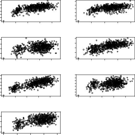
Figure 3.5 shows an example of decoy discrimination on the 4-state-reduced decoy set. This result is based on the residue-level packing and distance-dependent geometric potantial function discussed earlier. For all of the seven proteins in the 4-state-reduced set, the native structures have the lowest energy. In addition, all of

˚

the decoys with the lowest energy are within 2.5 A RMSD to the native structure. Table 3.2 lists the performance of the geometric potential function in fold-

ing and docking decoy discriminations. Several studies examine the comparative performance of different knowledge-based potential functions (Park and Levitt,

Table 3.2 Performance of geometric potential on folding and docking decoy discrimination

aNumber of native structures ranking first; e.g., 7/7 means seven out of seven native structures have the lowest energy among their corresponding decoy sets.

bz = E − Enative / ; E and are the mean and standard deviation of the energy values of conformations, respectively.

cNative complex is not included in these docking decoy sets. Thirty-two out of 42 decoy sets have at least one near-native

˚

structure (cRMSD < 2.5A) in the top 10 structures.

3.5.2 Protein–Protein Docking Prediction

Knowledge-based potential functions can also be used to study protein–protein interactions. Here we give an example of predicting the binding surface of seven antibody or antibody-related-proteins (e.g., Fab fragment, T-cell receptor) (Li and Liang, 2005a). These protein–protein complexes are taken from the 21 CAPRI (Critical Assessment of PRedicted Interactions) target proteins. CAPRI is a communitywide competition designed to objectively assess the abilities in protein–protein docking prediction (M´endez et al., 2005). In CAPRI, a blind docking prediction starts from two known crystallographic or NMR structures of unbound proteins and ends with a comparison to a solved structure of the protein complex, to which the participants did not have access. Knowledge-based potential functions, together with geometric complementarity potential functions, can be used to recognize near-native docking complexes and to guide the generation of conformations for protein–protein docking.

When docking two proteins together, we say a cargo protein is docked to a fixed seat protein. To determine the binding surfaces on the cargo protein, we can examine all possible surface patches on the unbound structure of cargo protein as candidate binding interfaces. The alpha knowledge-based potential function is then used to identify native or near native binding surfaces. To evaluate the performance of the potential function, we assume the knowledge of the binding interface on the seat protein. We further assume the knowledge of the degree of near neighbors for interface residues.

We first partition the surface of the unbound cargo protein into candidate surface patches, each having the same size as the native binding surface of m residues. A candidate surface patch is generated by starting from a surface residue on the cargo protein, and following alpha edges on the boundary of the alpha shape by breadth-first search, until m residues are found (Fig. 3.6a). We construct n candidate surface patches by starting in turn from each of the n surface residues on the cargo protein. Because each surface residue is the center of one of the n candidate surface

Fig. 3.6 Recognition of binding surface patch of CAPRI targets. (a) Boundary of alpha shape for a cargo protein. Each node represents a surface residue, and each edge represents the alpha edge between two surface residues. A candidate surface patch is generated by starting from a surface residue on the cargo protein, and following alpha edges on the boundary of the alpha shape by breadth-first search, until m residues are included. (b) Native interface and the surface patch with the best score on the antibody of the protein complex CAPRI Target T02. Only heavy chain (in red) and light chain (in blue) of the antibody are drawn. The antigen is omitted from this illustration for clarity. The best scored surface patch (in green) resembles the native interface (in yellow): 71% residues from this surface patch are indeed on the native binding interface. The residue in white is the starting residue used to generate this surface patch with the best score.

patches, the set of candidate surface patches covers exhaustively the whole protein binding interface.

Second, we assume that a candidate surface patch on the cargo protein has the same set of contacts as that of the native binding surface. The degree of near neighbors for each hypothetical contacting residue pair is also assumed to be the same. We replace the m residues of the native surface with the m residues from the

candidate surface patch. There are m! different ways to permute the m residues

20 m ! i =1 i

of the candidate surface patch, where mi is the number of residue type i on the candidate surface patch. A typical candidate surface patch has about 20 residues, therefore the number of possible permutations is very large. For each candidate surface patch, we take a sample of 5000 random permutations. For a candidate surface patch S Pi , we assume that the residues can be organized so that they can interact with the binding partner at the lowest energy. Therefore, the binding energy E (S Pi ) is estimated as

Here E (S Pi )k is calculated based on the residue-level packing and distancedependent potential for the k-th permutation. The value of E (S Pi ) is used to rank the candidate surface patches.