

Computational Methods for Protein Structure Prediction & Modeling V1 - Xu Xu and Liang
.pdf5 Protein Structure Comparison and Classification
Orhan C¸ amo˘glu and Ambuj K. Singh
5.1 Introduction
The success of genome projects has generated an enormous amount of sequence data. In order to realize the full value of the data, we need to understand its functional role and its evolutionary origin. Sequence comparison methods are incredibly valuable for this task. However, for sequences falling in the twilight zone (usually between 20 and 35% sequence similarity), we need to resort to structural alignment and comparison for a meaningful analysis. Such a structural approach can be used for classification of proteins, isolation of structural motifs, and discovery of drug targets.
The success of structural analysis rests on both the quality of the alignment of a query with a target protein and the speed with which relevant targets can be isolated in a large database. The multiple alignment of a set of protein structures denotes the extraction of their maximal common substructure. For such alignments to be computationally meaningful, the constraints of such approximate matching and a score function (or a distance measure) need to be defined.
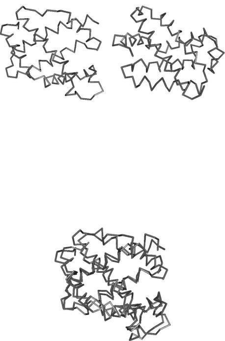
Comparison of protein structures is the basic building block of structural analysis. Structure comparison is carried out by first aligning two structures in 3D space and then assessing the similarity between them. For this alignment, two structures are superimposed onto each other. Figure 5.1 shows two protein structures from the Protein Data Bank (PDB) (Berman et al., 2000). The similarity between these two structures becomes evident after superimposition, as in Fig. 5.2.
Protein structure alignment of two protein structures P and Q is defined as a one-to-one mapping between the residues of P and Q. Using this mapping, two structures can be superimposed and a similarity measure between them can be computed. Alignment of protein structures is useful in answering a number of questions:
A protein with unknown function but known structure can be aligned to proteins with known functions and known structures. These alignments can provide clues regarding the function of the query protein.
Structural alignments can be used to classify proteins. Since the structure of a protein is strongly linked to its function, the resulting classifications can capture the functional and evolutionary similarity of proteins.
Multiple structure alignment of a set of proteins with a similar function can identify a structural motif pertaining to the function.
147
148 |
Orhan C¸ amo˘glu and Ambuj K. Singh |
a. |
b. |
Fig. 5.1 Backbone trace of (a) 1lh1 (leghemoglobin from yellow lupin) (b) 1urv-A (cytoglobin from human).
Remote homologies that are not apparent from sequence comparison can be discovered by structural alignment.
The exact alignment of protein structures is computationally expensive. This is due to the exponential number of correspondences between the point sets of two protein structures. [Once a correspondence has been found, the problem of aligning them in order to minimize the RMSD is quite fast—linear in the size of the proteins (Arun et al., 1987; Kabsch, 1978).] An early complexity result in this area is due to Lathrop (1994) who showed that the problem of protein threading (the alignment of a protein sequence to a protein structure) is NP-complete under variable-length gaps and nonlocal scoring functions.
Fig. 5.2 1urv-A is superimposed on 1lh1.
5. Protein Structure Comparison and Classification |
149 |
Goldman et al. (1999) have formulated the alignment problem using contact maps. A contact map of a protein structure is a graph in which nodes comprise the residues and edges are placed between two residues whose physical distances are below a given threshold. The alignment of two protein structures then amounts to finding the largest common subgraph of their contact maps. The authors show that even a simplified version of this problem (contact maps restricted to having a maximum degree of one) is hard to solve [NP-complete (Garey and Johnson, 1979)] and hard to approximate [MAXSNP-complete (Garey and Johnson, 1979)]. Approximate solutions within a factor of have also been investigated by Kolodny and Linial (2004). They show that if a scoring function similar to STRUCTAL (Levitt and Gerstein, 1998) is used, then an approximate solution can be found in time O(n10/ 6). Though exact approximation of the structural alignment problem is theoretically interesting, the currently available tools rely on heuristics. We focus on them in the remainder of the chapter.
The rest of the chapter is organized as follows. Section 5.2 discusses pairwise structure comparison and existing algorithms. Section 5.3 discusses multiple structure alignment and structural motifs. Section 5.4 presents techniques for querying protein structure databases. Section 5.5 presents classification of protein structures and automated classification techniques. Concluding remarks appear in Section 5.6. References and resources follow in Section 5.7. Some suggestions for further reading are included in Section 5.8.
5.2 Pairwise Alignment of Protein Structures
The goal of pairwise structure alignment is to find the best mapping between the residues of two given protein structures. The general methodology for achieving this can be summarized as follows.
1.Structure representation: Proteins have many characteristics including types of residues, positions of different atoms, types and properties of the various bonds. For the purposes of structural alignment, it is not feasible and usually not necessary to include all of these aspects in the representation of proteins. Many algorithms consider only 3D positions of a few atoms, and ignore their types. A further simplification can be obtained by considering only the positions of the backbone carbon atoms (C and C ). These are used to represent a residue. This reduces the number of atoms considered from thousands to hundreds for a typical protein.
2.Feature extraction: Most features for structure alignment are based on secondary structure elements (SSEs) and interresidue (inter-C or C ) distance matrices.
3.Structure comparison and alignment optimization: First, one finds similar features between two proteins (i.e., similar distance matrices for distance matrixbased methods or similar SSE layouts for geometric hashing-based methods). Sets of similar features define local alignments. These local alignments are then

150 |
Orhan C¸ amo˘glu and Ambuj K. Singh |
merged iteratively into a global alignment. This global alignment is optimized further.
4.Significance assessment: The significance of the obtained alignment is computed, usually by estimating the likelihood of obtaining a similar alignment at random. This estimate is based on protein similarity, alignment length, size of the proteins, and gaps in the alignment.
5.2.1Measuring the Quality of an Alignment
Given two proteins A and B, we are interested in identifying the largest common substructure of the proteins. A correspondence of size k identifies a subset of size k from each of the proteins and establishes an equivalence between the subsets. For example, if A = a1, a2, . . . , am and B = b1, b2, . . . , bn , then a correspondence of size five may be defined as (a1, a2, a3, a5, a6)–(b3, b4, b5, b6, b8). A correspondence is order preserving if it maintains the backbone order of C atoms. For example, the above correspondence is order preserving whereas the following correspondence is not: (a1, a2, a3, a5, a6)–(b3, b4, b7, b8, b5). In the order-preserving formulation, the problem of structure alignment simplifies to a 3D curve matching. The computational task becomes more difficult for non-order-preserving alignments. However, nonorder-preserving alignments are needed in order to discover non-sequential motifs such as molecular surface motifs and binding sites. They also allow a search of the database with partial structural information.
The similarity analysis of two protein structures is facilitated by rotations and translations so that the common substructures of the proteins are juxtaposed. Such rigid body transformations have been studied in detail in computer vision (Arun et al., 1987). Given a protein A, we denote its rigid body transformation using a mapping f as f (A).
The root-mean-square distance (RMSD) between two proteins A and B under a correspondence R of size k and a transformation f is defined as
RMSD(A,B, R, f ) |
|
|
|
|
i=1 dist (ki |
i |
|
|
= |
|
|
|
k |
2 a |
, f (R(a ))) |
|
|
|
|
|
|
||
Given two proteins and a correspondence between them, it is computationally easy to find the transformation that minimizes the RMSD. RMSD between two proteins A and B under a correspondence R of size k is defined as RMSD(A, B, R) = argmin f RMSD(A, B, R, f ).
Another measure of distance between protein structures is defined using the interresidue distances directly (and without using any rigid body transformations). This distance, distance matrix error (DME), is defined as DME(A, B, R) =
N |
|
|
|
|
|
|
|
|
|
|
i=1 |
|
j=1 |
(dist |
(ai , a j ) − dist |
(R(ai ), R(a j ))). The advantage of this repre- |
|||
1 |
|
|
k |
|
k |
2 |
2 |
|
|
sentation is that two structures do not need to be superimposed and the measure can be computed directly using the distance matrices.

5. Protein Structure Comparison and Classification |
151 |
The interplay between the RMSD and the size of the identified common substructure is interesting. Since RMSD is an average measure, it decreases monotonically with the size of the common substructure. However, small alignments may not be meaningful. Irving et al. (2001) analyzed the variation of RMSD with the number of aligned residues. They found a linear dependence of RMSD on the number of residues for a small number of aligned residues followed by an exponential region.
Some researchers have defined distance measures so that the effect of distant pairs is reduced. For example, DALI (Holm and Sander, 1993) uses an elastic score defined as follows:
|
|
E |
|
|diAj −diBj |
| |
|
w(d ) i |
|
j |
|
|
|
|
|
|
|
|||||
E (i, j) |
|
− di j |
|
i |
= |
j |
(5.1) |
|||
|
= |
E |
|
|
|
|
|
= |
|
|
|
|
|
|
|
|
|
|
|
|
|
where diAj and diBj are the equivalenced elements in the distance matrices of proteins A and B, di j is the average of diAj and diBj , E = 0.20, and envelope function w is defined as w(r ) = exp(−r 2/400). The envelope function gives lower weights to residues that are farther apart, thus reducing their relative contribution.
In a similar vein, Levitt and Gerstein (1998) defined a scoring scheme that depends more on the best-fitting residues. In this scheme, a scoring matrix is created based on an initial alignment of proteins. The score for each entry is defined as
Si, j = M 2 where di j is the distance between residues i and j, M = 20, and
di j
d0
al. (2004) proposed a new scoring scheme for CE. CE score is defined by
r msd |
1 + |
num |
|
gap |
where and are greater than 0. The significance |
|||
|
||||||||
aligned |
|
length |
aligned |
|
length |
|||
of an observed score is computed by using the probability density function for the random scores.
Overall, the similarity of two protein structures is difficult to quantify using a number. Godzik (1996) investigated the alignment of a number of protein pairs and found that although different alignment methods produce similar results at the SSE level, there are significant differences at the residue level. The RMSD values and the length of aligned substructures varied widely. For example, the alignment of azurin (1azcA) and plastocyanin (1plc) produced RMSD in the range of 1.5–6.7 A˚ and the length of aligned substructures varied in the range of 13–108 residues. There is usually no unique answer to the structural alignment problem and additional input is required to characterize a good solution (e.g., in a given pair of proteins, one may want to focus more on the well-conserved core and less on the loop regions).
Once a set of similar candidates has been obtained by using a database search, the statistical distribution of similarity scores needs to be computed in order to assign a level of significance ( p-value). It is difficult to distinguish between structure similarities that arise from evolutionary relationships and those resulting from
152 |
Orhan C¸ amo˘glu and Ambuj K. Singh |
physical constraints on protein folding. However, the question of significance can be answered in a purely mathematical manner by considering the space of possible configurations, the size of the alignment, and the distribution of the scores (Gibrat et al., 1996; Ye and Godzik, 2004; Holm and Sander, 1993; Shindyalov and Bourne, 1998).
5.2.2Computational Approaches
Many methods have been proposed for pairwise protein structure comparison. [Excellent in-depth surveys can be found in Eidhammer et al. (2000) and Brown et al. (1996).] These methods propose different approximations and approaches to structure alignment. They use different types of representations (atoms, residues, secondary structure elements and groups of these) and algorithms (dynamic programming, geometric hashing, randomized algorithms). These methods are grouped based on their data representations and algorithms.
5.2.2.1 Dynamic Programming-Based Approaches
Dynamic programming (DP) algorithms have been used to find the optimal sequence alignment between pairs of sequences (Needleman and Wunsch, 1970). In structural alignment, however, the traditional DP algorithm cannot be used directly. The difference is that in structure alignment, the distance between two residues is dependent on the alignment of other residues. Sali and Blundell (1990) managed to overcome this difficulty by using rotationand transformation-independent features on the scoring function. Employing simulated annealing, they first find possible equivalences between two proteins depending on a set of residue properties (sequence identity, hydrophobicity, charge, volume, torsional angles). Similarity of residue properties is then used to create a two-dimensional similarity matrix. Finally, the proteins are aligned by applying dynamic programming.
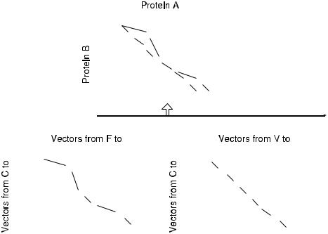
Orengo and Taylor (1996) proposed SSAP that uses two levels of dynamic programming (double dynamic programming). In the upper-level dynamic programming, score matrix entry Si j represents the score of aligning the ith residue of the first protein to the jth residue of the second protein. The best path in this matrix finds the optimal alignment of the two proteins. The value Si j is computed at the lower level of dynamic programming: the ith and jth residues are assumed to be aligned, and a score matrix is computed by using the difference of C –C vectors of residues. The resulting score Si j represents how well the rest of the residues are aligned when the ith and jth residues are aligned.
An example of two levels of dynamic programming is given in Fig. 5.3. In the first lower level matrix, residue C of protein B is aligned to residue F of protein A. To obtain the matrix, C –C vectors from residue C to each residue in protein B are compared to C –C vectors from residue F to each residue in protein A. The best scoring path is identified in the score matrix. Scores in this path are copied to the main score matrix in the upper level. The second score matrix in the lower level is
5. Protein Structure Comparison and Classification |
153 |
|||||||||||||||||||||||||
|
|
|
|
|
|
|
|
|
|
|
|
|
|
|
|
|
|
|
|
|
|
|
|
|
|
|
|
|
|
|
|
|
|
|
|
|
|
|
|
|
|
|
|
|
|
|
|
|
|
|
|
|
|
|
|
|
|
|
|
|
|
|
|
|
|
|
|
|
|
|
|
|
|
|
|
|
|
|
|
|
|
|
|
|
|
|
|
|
|
|
|
|
|
|
|
|
|
|
|
|
|
|
|
|
|
|
|
|
|
|
|
|
|
|
|
|
|
|
|
|
|
|
|
|
|
|
|
|
|
|
|
|
|
|
|
|
|
|
|
|
|
|
|
|
|
|
|
|
|
|
|
|
|
|
|
|
|
|
|
|
|
|
|
|
|
|
|
|
|
|
|
|
|
|
|
|
|
|
|
|
|
|
|
|
|
|
|
|
|
|
|
|
|
|
|
|
|
|
|
|
|
|
|
|
|
|
|
|
|
|
|
|
|
|
|
|
|
|
|
|
|
|
|
|
|
|
|
|
|
|
|
|
|
|
|
|
|
|
|
|
|
|
|
|
|
|
|
|
|
|
|
|
|
|
|
|
|
|
|
|
|
|
|
|
|
|
|
|
|
|
|
|
|
|
|
|
|
|
|
|
|
|
|
|
|
|
|
|
|
|
|
|
|
|
|
|
|
|
|
|
|
|
|
|
|
|
|
|
|
|
|
|
|
|
|
|
|
|
|
|
|
|
|
|
|
|
|
|
|
|
|
|
|
|
|
|
|
|
|
|
|
|
|
|
|
|
|
|
|
|
|
|
|
|
|
|
|
|
|
|
|
|
|
|
|
|
|
|
|
|
|
|
|
|
|
|
|
|
|
|
|
|
|
|
|
|
|
|
|
|
|
|
|
|
|
|
|
|
|
|
|
|
|
|
|
|
|
|
|
|
|
|
|
|
|
|
|
|
|
|
|
|
|
|
|
|
|
|
|
|
|
|
|
|
|
|
|
|
|
|
|
|
|
|
|
|
|
|
|
|
|
|
|
|
|
|
|
|
|
|
|
|
|
|
|
|
|
|
|
|
|
|
|
|
|
|
|
|
|
|
|
|
|
|
|
|
|
|
|
|
|
|
|
|
|
|
|
|
|
|
|
|
|
|
|
|
|
|
|
|
|
|
|
|
|
|
|
|
|
|
|
|
|
|
|
|
|
|
|
|
|
|
|
|
|
|
|
|
|
Fig. 5.3 SSAP algorithm uses two levels of dynamic programming. Lower level scoring matrices are calculated by aligning one residue from each structure. Then, C vectors relative to the aligned residues are compared to fill out lower level score matrix. The best path is computed and aggregated to the upper level (Orengo and Taylor, 1996).
computed by aligning residue C of protein B to residue V of protein A while using C –C vectors from residue C in protein B and from residue V in protein A. The best path is identified and copied to the main score matrix. After all lower matrices are processed, the best scoring path in the upper level scoring matrix is found by dynamic programming. This path defines the alignment between proteins.
Taylor (1999) proposed an extension to the SSAP algorithm by incorporating a stochastic component: suboptimal alignments are allowed and double dynamic programming is used to evaluate the effect of these suboptimal alignments iteratively.
Gerstein and Levitt (1996) proposed another approach to iterative dynamic programming. They start with a random alignment. Given an alignment, they optimize the RMSD by superimposing the proteins, and compute the interresidue distances. Dynamic programming is applied to the interresidue distance matrix to find the best residue correspondences. The current alignment is then modified using these correspondences. This procedure is repeated until convergence. The entire computation is carried out with different initial alignments and the best resulting alignment is reported.
One major drawback of dynamic programming-based approaches is that they preserve the sequence order of residues in the structural alignment. These sequential
154 |
Orhan C¸ amo˘glu and Ambuj K. Singh |
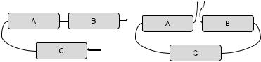
Fig. 5.4 Same layout of SSE structures can have different sequence orders due to circular mutations. The layout on the left has a C AB order on the SSEs while the layout on the right has a BC A order (Binkowski et al., 2004).
alignments cannot capture similarities between proteins where circular permutations have occurred. Two proteins with a similar structure layout of SSEs can have different sequence layouts of SSEs. In Fig. 5.4, SSEs A, B, and C have similar structural layouts in both of the proteins. However, their sequence orders are significantly different. The sequence order for the first protein is CAB whereas it is BCA for the second protein. To discover such structural similarities where sequence order is not preserved, a number of algorithms have been proposed. We elaborate on some of them.
5.2.2.2 Distance Matrices and Contact Maps
Algorithms in this category represent protein structures as two-dimensional distance matrices. For each residue in a protein, its distances to the remaining residues are computed to construct these matrices. DALI (Holm and Sander, 1993), one of the most popular algorithms, uses the distance matrices to find highly similar local structures. The intuition is that if two protein structures are similar, then their distance matrices should be similar too. In the first step of the algorithm, similar submatrices of size six in two proteins are found by comparing their distance matrices. These comparisons result in alignments of size six between two proteins. Then, compatible alignments are merged to obtain larger alignments called seeds. These seeds are randomly merged and extended by making optimal and suboptimal choices via a Monte Carlo algorithm. The best alignments are further improved by randomly removing parts of the alignment and realigning the proteins.
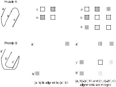
An example of merging of compatible alignments is shown in Fig. 5.5. Upon comparison of distance matrices of proteins A and B, matrix component (a, b) is aligned to (a , b ). Similarly, (b, c) is aligned to (b , c ). Since these two alignments are overlapping (i.e., they both align b to b ), they are checked for compatibility. If the nine matrix components for these two alignments are found similar to each other, alignments are merged to obtain a seed of (a, b, c) − (a , b , c ).
Two different measures of scoring are used in DALI: a rigid body similarity measure and an elastic scoring measure. This approach does not require the alignments to be order preserving. In recent versions of DALI, the computational performance has been improved by imposing SSE constraints on the alignments.
5. Protein Structure Comparison and Classification |
155 |
|||||||||||||||||
|
|
|
|
|
|
|
|
|
|
|
|
|
|
|
|
|
|
|
|
|
|
|
|
|
|
|
|
|
|
|
|
|
|
|
|
|
|
|
|
|
|
|
|
|
|
|
|
|
|
|
|
|
|
|
|
|
|
|
|
|
|
|
|
|
|
|
|
|
|
|
|
|
|
|
|
|
|
|
|
|
|
|
|
|
|
|
|
|
|
|
|
|
|
|
|
|
|
|
|
|
|
|
|
|
|
|
|
|
|
|
|
|
|
|
|
|
|
|
|
|
|
|
|
|
|
|
|
|
|
|
|
|
|
|
|
|
|
|
|
|
|
|
|
|
|
|
|
|
|
|
|
|
|
|
|
|
|
|
|
|
|
|
|
|
|
|
|
|
|
|
|
|
|
|
|
|
|
|
|
|
|
|
|
|
|
|
|
|
|
|
|
|
|
|
|
|
|
|
|
|
|
|
|
|
|
|
|
|
|
|
|
|
|
|
|
|
|
|
|
|
|
|
|
|
|
|
|
Fig. 5.5 DALI algorithm first aligns small parts of each protein. First (a, b) is aligned to (a , b )
and (b, c) is aligned to (b , c ). These two alignments are merged to obtain a larger alignment (a, b, c) − (a , b , c ) (Holm and Sander, 1993).
CE (Shindyalov and Bourne, 1998) uses distance matrices to find small but highly similar fragments in a manner similar to DALI. The difference is that CE uses a combinatorial extension of these fragments. In the first stage, all combinations of 8 residue alignments between two proteins are tested and ones that meet a threshold are selected. Then starting from a fragment, the alignment is extended by adding new fragments. A new fragment is added if its addition will result in a better alignment score than some threshold. To improve the performance, the program does not allow gaps of length larger than 30 residues. After the best alignments of fragments are found, they are further improved by using a dynamic programming approach.
Chew et al. (1999) represent a protein structure by vectors defined by adjacent C atoms. These vectors represent the protein backbone. They place these vectors on a unit sphere and compare two proteins by their trace on this sphere.
5.2.2.3 Geometric Hashing
Geometric hashing allows rotation and translation invariant comparison of 3D objects. Nussinov and Wolfson (1991) adapt this idea for the comparison of protein structures. Their approach is to use a set of reference frames for each protein and map its residues into 3D grid cells for each reference frame. If two protein structures are similar, then there exists a pair of reference frames (one for each protein) such that a large number of residue pairs will be mapped to the same grid cell. A hash function can be associated with the grid cells, allowing efficient lookup. A reference
156 |
Orhan C¸ amo˘glu and Ambuj K. Singh |
frame can be defined using C , C , and N atoms of each residue (Pennec and Ayache, 1998), or using three or more residues at a time.
Holm and Sander (1995) use geometric hashing on the secondary structure elements. Reference frames are defined for pairs of SSEs. Based on each frame, the locations of the rest of the SSEs are hashed. A pair of frames that maps corresponding SSEs into similar locations is found. Such a matching frame forms an initial alignment that is refined by an iterative process.
Proteins are flexible molecules capable of undergoing structural conformations such as hinge-based motion (Rose and Stroud, 1998). Incorporation of such flexibility implies moving away from the common assumptions of proteins as rigid bodies. Some tools have been developed recently (Shatsky, 2004; Ye and Godzik, 2003) that incorporate flexible alignments. Verbitsky et al. (1999) use geometric hashing to align structures allowing hinge bending.
5.2.2.4 Hierarchical Algorithms
Hierarchical algorithms are based on rapidly identifying mappings between similar SSE fragments of two proteins. The similarity of two fragments is defined using length and angle constraints. Fragment pairs that align well form the seed for expensive residue-level alignments.
The VAST program (Madej et al., 1995) carries out a hierarchical alignment using SSEs. It begins with a bipartite graph: vertices on one side consist of pairs of SSEs from the query protein and vertices on the other side consist of pairs of SSEs from the target protein. An edge is inserted between two pairs of SSEs if they can be aligned well. A maximal clique is found in this bipartite graph; this defines the initial SSE alignment. This initial alignment is extended to C atoms by Gibbs sampling. A nice feature of the VAST program is its ability to report on the unexpectedness of the match through a p-value. This is computed by considering the size of the match, the size of the proteins, and the quality of the alignment.
A number of other algorithms also use hierarchical alignment (Alexandrov and Fischer, 1996; Singh and Brutlag, 1997; Holm and Sander, 1995). LOCK (Singh and Brutlag, 1997) represents SSEs by vectors and matches pairs of SSEs based on similarity of angles and distances between them. The alignment of SSEs is extended using iterative dynamic programming. Proteins are aligned and the nearest neighbor of each residue on the other structure is computed. The residue pairs that identify each other as the nearest neighbor define the new alignment. This process is repeated until convergence.
Novotny et al. (2004) evaluated various pairwise structure comparison tools for identification of similar folds. The CATH (Orengo et al., 1997) structure classification database was used as a reference. None of the tools were able to achieve a 100% success rate, but CE, DALI, and VAST showed best performance. Sierk and Pearson (2004) performed a similar analysis to evaluate the performance of comparison tools in detecting homologues. They showed that DALI was more selective than the other tools.