Computational Methods for Protein Structure Prediction & Modeling V1 - Xu Xu and Liang

a b c

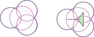
Fig. 6.3 The family of alpha shapes or dual simplicial complexes for a two-dimensional toy molecule. (a) We collect simplices from the Delaunay triangulation as atoms grow by increasing the value. At the beginning as grows from −∞, atoms are in isolation and we only have vertices in the alpha shape. (b, c) When is increased such that some atom pairs start to intersect, we collect the corresponding Delaunay edges. (d) When three atoms intersect as increases, we collect the corresponding Delaunay triangles. When = 0, the collection of vertices, edges, and triangles form the dual simplicial complex K0, reflecting the topological structure of the protein molecule. (e) More edges and triangles from the Delaunay triangulation are now collected as atoms continue to grow. (d) Finally, all vertices, edges, and triangles are now collected as atoms are grown to large enough size. We get back the full original Delaunay complex.

any specific value, we have a dual simplicial complex or alpha complex K formed by the collected simplices. If all atoms take the incremented radius of ri + rs and= 0, we have the dual simplicial complex K0 of the protein molecule. When is sufficiently large, we have collected all simplices and we get the full Delaunay complex. This series of simplicial complexes at different value form a family of shapes (Fig. 6.3), called alpha shapes, each faithfully representing the geometric and topological property of the protein molecule at a particular resolution parametrized by the value.

An equivalent way to obtain the alpha shape at = 0 is to take a subset of the simplices, with the requirement that the corresponding intersections of Voronoi cells must overlap with the body of the union of the balls. We obtain the dual complex or alpha shape K0 of the molecule at = 0 (Fig. 6.2c):

Alpha shape provides a guide map for computing geometric properties of the structures of biomolecules. Take the molecular surface as an example; the reentrant surfaces are formed by the concave spherical patch and the toroidal surface. These can be mapped from the boundary triangles and boundary edges of the alpha shape, respectively (Edelsbrunner et al., 1995). Recall that a triangle in the Delaunay tetrahedrization corresponds to the intersection of three Voronoi regions, i.e., a Voronoi edge. For a triangle on the boundary of the alpha shape, the corresponding Voronoi

edge intersects with the body of the union of balls by definition. In this case, it intersects with the solvent-accessible surface at the common intersecting vertex when the three atoms overlap. This vertex corresponds to a concave spherical surface patch in the molecular surface. For an edge on the boundary of the alpha shape, the corresponding Voronoi plane coincides with the intersecting plane when two atoms meet, which intersect with the surface of the union of balls on an arc. This line segment corresponds to a toroidal surface patch. The remaining parts of the surface are convex pieces, which correspond to the vertices, namely, the atoms on the boundary of the alpha shape.

The numbers of toroidal pieces and concave spherical pieces are exactly the numbers of boundary edges and boundary triangles in the alpha shape, respectively. Because of the restriction of bond length and the excluded volume effects, the number of edges and triangles in molecules are roughly on the order of O(n) (Liang et al., 1998a).

6.2.5Metric Measurement

We have described the relationship between the simplices and the surface elements of the molecule. Based on this relationship, we can compute efficiently size properties of the molecule. We take the problem of volume computation as an example.

Consider a grossly incorrect way to compute the volume of a protein molecule using the solvent-accessible surface model. We could define that the volume of the molecule is the summation of the volumes of individual atoms, whose radii are inflated to account for the solvent probe. By doing so we would have significantly exaggerated the value of the true volume, because we neglected to consider volume overlaps. We can explicitly correct this by following the inclusion–exclusion formula: when two atoms overlap, we subtract the overlap; when three atoms overlap, we first subtract the pair overlaps, we then add back the triple overlap, etc. This continues when there are four, five, or more atoms intersecting. At the combinatorial level, the principle of inclusion–exclusion is related to the Gauss–Bonnet theorem used by Connolly (Connolly, 1983). The corrected volume V (B) for a set of atom balls B can then be written as

V (B) = (−1)dim(T )−1vol T , (6.4)

vol( T )>0

T B

where vol( T ) represents volume overlap of various degree, and T B is a subset

of the balls with nonzero volume overlap: vol( T ) > 0.

However, the straightforward application of this inclusion–exclusion formula does not work well. The degree of overlap can be very high: theoretical and simulation studies showed that the volume overlap can be up to 7–8 degrees (Kratky, 1981; Petitjean, 1994). It is difficult to keep track of these high degree of volume overlaps

Fig. 6.4 An example of analytical area calculation. (A) Area can be computed using the direct inclusion-exclusion. (B) The formula is simplified without any redundant terms when using alpha shape.

correctly during computation, and it is also difficult to compute the volume of these overlaps because there are many different combinatorial situations, i.e., to quantify how large is the k-volume overlap of which one of the k7 or k8 overlapping atoms for all of k = 2, . . . , 7 (Petitjean, 1994). It turns out that for three-dimensional molecules, overlaps of five or more atoms at a time can always be reduced to a “+” or a “−” signed combination of overlaps of four or fewer atom balls (Edelsbrunner, 1995). This requires that the 2-body, 3-body, and 4-body terms in Eq. (6.4) enter the formula if and only if the corresponding edge i j connecting the two balls (1-simplex), triangles i jk spanning the three balls (2-simplex), and tetrahedron i jkl cornered on the four balls (3-simplex) all exist in the dual simplicial complex K0 of the molecule (Edelsbrunner, 1995; Liang et al., 1998a). Atoms corresponding to these simplices will all have volume overlaps. In this case, we have the simplified exact expansion:

The same idea is applicable for the calculation of surface area of molecules.

An example: An example of area computation by alpha shape is shown in Fig. 6.4. Let b1, b2, b3, b4 be the four disks. To simplify the notation we write Ai for the area of bi , Ai j for the area of bi ∩ b j , and Ai jk for the area of bi ∩ b j ∩ bk . The total area of the union, b1 b2 b3 b4, is

Atotal = ( A1 + A2 + A3 + A4)

− ( A12 + A23 + A24 + A34)

+ A234.

We add the area of bi if the corresponding vertex belongs to the alpha complex (Fig. 6.4), we subtract the area of bi ∩ b j if the corresponding edge belongs to the alpha complex, and we add the area of bi ∩ b j ∩ bk if the corresponding triangle belongs to the alpha complex. Note without the guidance of the alpha complex, the inclusion–exclusion formula may be written as

Atotal = ( A1 + A2 + A3 + A4)

−( A12 + A13 + A14 + A23 + A24 + A34) + ( A123 + A124 + A134 + A234)

−A1234.

This contains six canceling redundant terms: A13 = A123, A14 = A124, and A134 = A1234. Computing these terms would be wasteful. Such redundancy does not occur when we use the alpha complex: the part of the Voronoi regions contained in the respective atom balls for the redundant terms do not intersect. Therefore, the corresponding edges and triangles do not enter the alpha complex. In two dimensions, we have terms of at most three disk intersections, corresponding to triangles in the alpha complex. Similarly, in three dimensions the most complicated terms are intersections of four spherical balls, and they correspond to tetrahedra in the alpha complex.

Voids and pockets: Voids and pockets represent the concave regions of a protein surface. Because shape-complementarity is the basis of many molecular recognition processes, binding and other activities frequently occur in pocket or void regions of protein structures. For example, the majority of enzyme reactions take place in surface pockets or interior voids.

The topological structure of the alpha shape also offers an effective method for computing voids and pockets in proteins. Consider the Delaunay tetrahedra that are not included in the alpha shape. If we repeatedly merge any two such tetrahedra on the condition that they share a 2-simplex triangle, we will end up with discrete sets of tetrahedra. Some of them will be completely isolated from the outside, and some of them are connected to the outside by triangle(s) on the boundary of the alpha shape. The former corresponds to voids (or cavities) in proteins, the latter corresponds to pockets and depressions in proteins.

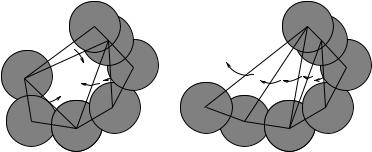
A pocket differs from a depression in that it must have an opening that is at least narrower than one interior cross section. Formally, the discrete flow (Edelsbrunner et al., 1998) explains the distinction between a depression and a pocket. In a twodimensional Delaunay triangulation, the empty triangles that are not part of the alpha shape can be classified into obtuse triangles and acute triangles. The largest angle of an obtuse triangle is more than 90 degrees, and the largest angle of an acute triangle is less than 90 degrees. An empty obtuse triangle can be regarded as a “source” of empty space that “flows” to its neighbor, and an empty acute triangle a “sink” that collects flow from its obtuse empty neighboring triangle(s). In Fig. 6.5a, obtuse triangles 1, 3, 4, and 5 flow to the acute triangle 2, which is a sink. Each of the discrete

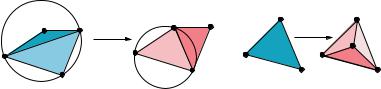
Fig. 6.6 An illustration of locally Delaunay edge and flips. (a) For the quadrilateral abcd, edge ab is not locally Delaunay, as the circumcircle passing through edge ab and a third point c contains a fourth point d. Edge cd is locally Delaunay, as b is outside the circumcircle adc. An edge-flip or 2-to-2 flip replaces edge ab by edge cd, and replace the original two triangles abc and adb with two new triangles acd and bcd. (b) When a new vertex is inserted, we replace the old triangle containing this new vertex with three new triangles. This is called 1-to-3 flips.

for a set of atoms of different radii. For simplicity, we sketch the outline of the algorithm below for two-dimensional unweighted Delaunay triangulation.

The intuitive idea of the algorithm can be traced back to the original observation of Delaunay. For the Delaunay triangulation of a point set, the circumcircle of an edge and a third point forming a Delaunay triangle must not contain a fourth point. Delaunay showed that if all edges in a particular triangulation satisfy this condition, the triangulation is a Delaunay triangulation. It is easy to come up with an arbitrary triangulation for a point set. A simple algorithm to covert this triangulation to the Delaunay triangulation is therefore to go through each of the triangles, and make corrections using “flips” discussed below, if a specific triangle contains an edge violating the above condition. The basic ingredients for computing Delaunay tetrahedrization are generalizations of these observations. We discuss the concept of locally Delaunay edge and the edge-flip primitive operation below.

Locally Delaunay edge. We say an edge ab is locally Delaunay if either it is on the boundary of the convex hull of the point set, or if it belongs to two triangles abc and abd, and the circumcircle of abc does not contain d (e.g., edge cd in Fig. 6.6a).

Edge-flip. If ab is not locally Delaunay (edge ab in Fig. 6.6a), then the union of the two triangles abc abd is a convex quadrangle acbd, and edge cd is locally Delaunay. We can replace edge ab by edge cd. We call this an edge-flip or 2-to-2 flip, as two old triangles are replaced by two new triangles.

We recursively check each boundary edge of the quadrangle abcd to see if it is also locally Delaunay after replacing ab by cd. If not, we recursively edge-flip it.

Incremental algorithm for Delaunay triangulation. Assume we have a finite set of points (namely, atom centers) S = {z1, z2, . . . , zi , . . . , zn }. We start with a large auxiliary triangle that contains all these points. We insert the points one by one. At all times, we maintain a Delaunay triangulation Di up to insertion of point zi .

After inserting point zi , we search for the triangle i−1 that contains this new point. We then add zi to the triangulation and split the original triangle i−1 into three smaller triangles. This split is called 1-to-3 flip, as it replaces one old triangle with three new triangles. We then check if each of the three edges in i−1 still satisfies

Algorithm 1 Delaunay triangulation

Obtain random ordering of points {z1, . . . , zn }; for i = 1 to n do

find i−1 such zi i−1;

add zi , and split i−1 into three triangles (1-to-3 flip); while any edge ab not locally Delaunay do

flip ab to other diagonal cd (2-to-2 edge flip); end while

end for

the locally Delaunay requirement. If not, we perform a recursive edge-flip. This algorithm is summarized in Algorithm 1.

In R3, the algorithm of tetrahedrization becomes more complex, but the same basic ideas apply. In this case, we need to locate a tetrahedron instead of a triangle that contains the newly inserted point. The concept of locally Delaunay is replaced by the concept of locally convex, and there are flips different than the 2-to-2 flip in R3 (Edelsbrunner and Shah, 1996). Although an incremental approach, i.e., sequentially adding points, is not necessary for Delaunay triangulation in R2, it is necessary in R3 to avoid nonflippable cases and to guarantee that the algorithm will terminate. This incremental algorithm has excellent expected performance (Edelsbrunner and Shah, 1996).

The computation of Voronoi diagram is conceptually easy once the Delaunay triangulation is available. We can take advantage of the mathematical duality and compute all of the Voronoi vertices, edges, and planar faces from the Delaunay tetrahedra, triangles, and edges. Because one point zi may be a vertex of many Delaunay tetrahedra, the Voronoi region of zi therefore may contain many Voronoi vertices, edges, and planar faces. The efficient quad-edge data structure can be used for software implementation (Guibas and Stolfi, 1985).

Volume and area computation: Let V and A denote the volume and area of the molecule, respectively, K0 for the alpha complex, for a simplex in K, i for a vertex, i j for an edge, i jk for a triangle, and i jkl for a tetrahedron. The algorithm for volume and area computation can be written as Algorithm 2. Additional details of volume and area computation can be found in Edelsbrunner et al. (1995), and Liang et al. (1998a).

Software: The software package Delcx for computing weighted Delaunay tetrahedrization, Mkalf for computing the alpha shape, Volbl for computing volume and area of both molecules and interior voids can be found at www.alphashape.org. The CASTp webserver for pocket computation can be found at cast.engr.uic.edu. There are other studies that compute or use Voronoi diagrams of protein structures

194 Jie Liang

Algorithm 2 Volume and area measurement

V := A := 0.0; for all K do

if is a vertex i then

V := V + vol(bi ) ; A := A + area(bi ); end if

if is an edge ij then

(Chakravarty et al., 2002; Goede et al., 1997; Harpaz et al., 1994), although not all computes the weighted version which allows atoms to have different radii.

In this short description of algorithm, we have neglected many details important for geometric computation, for example, the problem of how to handle geometric degeneracy, namely, when three points are colinear, or when four points are coplanar. Interested readers should consult the excellent monograph by Edelsbrunner for a detailed treatise of these and other important topics in computational geometry (Edelsbrunner, 2001).

6.4 Applications: Packing Analysis

An important application of the Voronoi diagram and volume calculation is the measurement of protein packing. Tight packing is an important feature of protein structure (Richards, 1974a, 1977), and is thought to play important roles in protein stability and folding dynamics (Levitt et al., 1997). The packing density of a protein is measured by the ratio of its van der Waals volume and the volume of the space it occupies. One approach is to calculate the packing density of buried residues and atoms using Voronoi diagram (Richards, 1974a, 1977). This approach was also used to derive parameters of radii of atoms (Tsai et al., 1999).

Based on the computation of voids and pockets in proteins, a detailed study surveying major representatives of all known protein structural folds showed that there is a substantial amount of voids and pockets in proteins (Liang and Dill, 2001). On average, every 15 residues introduces a void or a pocket (Fig. 6.7a). For a perfectly solid three-dimensional sphere of radius r, the relationship between volume V = 4 r 3/3 and surface area A = 4 r 2 is: V A3/2. In contrast, Fig. 6.7b shows that the van der Waals volume scales linearly with the van der Waals surface areas

Fig. 6.7 Voids and pockets for a set of 636 proteins representing most of the known protein folds, and the scaling behavior of the geometric properties of proteins. (a) The number of voids and

˚

pockets detected with a 1.4 A probe is linearly correlated with the number of residues in a protein. Only proteins with less than 1,000 residues are shown. Solid triangles and empty circles represent the pockets and the voids, respectively. (b) The van der Waals volume and van der Waals area of proteins scale linearly with each other. Similarly, molecular surface volume also scales linearly

˚

with molecular surface area using a probe radius of 1.4 A. (Data not shown. Figure adapted after Liang and Dill, 2001).

of proteins. The same linear relationship holds irrespective of whether we relate molecular surface volume and molecular surface area, or solvent-accessible volume and solvent-accessible surface area. This and other scaling behavior point out that the protein interior is not packed as tight as solid (Liang and Dill, 2001). Rather, packing defects in the form of voids and pockets are common in proteins.

If voids and pockets are prevalent in proteins, an interesting question is what is the origin of the existence of these voids and pockets. This question was studied by examining the scaling behavior of packing density and coordination number of residues through the computation of voids, pockets, and edge simplices in the alpha shapes of random compact chain polymers (Zhang et al., 2003). For this purpose, a 32-state discrete state model was used to generate a large ensemble of compact self-avoiding walks. This is a difficult task, as it is very challenging to generate a large number of independent conformations of very compact chains that are selfavoiding. The results in Zhang et al. (2003) showed that it is easy for compact random chain polymers to have similar scaling behavior of packing density and coordination number with chain length. This suggests that proteins are not optimized by evolution to eliminate voids and pockets, and the existence of many pockets and voids is random in nature, due to the generic requirement of compact chain polymers. The frequent occurrence and the origin of voids and pockets in protein structures raise a challenging question: How can we distinguish voids and pockets that perform biological functions such as binding from those formed by random chance? This question is related to the general problem of protein function prediction.

6.5Applications: Protein Function Prediction from Structures

Conservation of protein structures often reveals very distant evolutionary relationships, which are otherwise difficult to detect by sequence analysis (Todd et al., 2001). Comparing protein structures can provide insightful ideas about the biochemical functions of proteins (e.g., active sites, catalytic residues, and substrate interactions) (Holm and Sander, 1997; Martin et al., 1998; Orengo et al., 1999).

A fundamental challenge in inferring protein function from structure is that the functional surface of a protein often involves only a small number of key residues. These interacting residues are dispersed in diverse regions of the primary sequences and are difficult to detect if the only information available is the primary sequence. Discovery of local spatial motifs from structures that are functionally relevant has been the focus of many studies.

Graph-based methods for spatial patterns in proteins: To analyze local spatial patterns in proteins. Artymiuk et al. developed an algorithm based on subgraph isomorphism detection (Artymiuk et al., 1994). By representing residue side chains as simplified pseudo-atoms, a molecular graph is constructed to represent the patterns of side-chain pseudo-atoms and their interatomic distances. A user-defined query pattern can then be searched rapidly against the Protein Data Bank for similarity relationship. Another widely used approach is the method of geometric hashing. By examining spatial patterns of atoms, Fischer et al. developed an algorithm that can detect surface similarity of proteins (Fischer et al., 1982; Norel et al., 1994). This method has also been applied by Wallace et al. for the derivation and matching of spatial templates (Wallace et al., 1997). Russell developed a different algorithm that detects side-chain geometric patterns common to two protein structures (Russell, 1998). With the evaluation of statistical significance of measured root-mean-square distance, several new examples of convergent evolution were discovered, where common patterns of side chains were found to reside on different tertiary folds.

These methods have a number of limitations. Most require a user-defined template motif, restricting their utility for automated database-wide search. In addition, the size of the spatial pattern related to protein function is also often restricted.

Predicting protein functions by matching pocket surfaces: Protein functional surfaces are frequently associated with surface regions of prominent concavity (Laskowski et al., 1996; Liang et al., 1998c). These include pockets and voids, which can be accurately computed as we have discussed. Computationally, one wishes to automatically identify voids and pockets on protein structures where interactions exist with other molecules such as substrates, ions, ligands, or other proteins.

Binkowski et al. developed a method for predicting protein function by matching a surface pocket or void on a protein of unknown or undetermined function to the pocket or void of a protein of known function (Binkowski et al., 2003a, 2005). Initially, the Delaunay tetrahedrization and alpha shapes for almost all of the structures