Biomechanics Principles and Applications - Schneck and Bronzino

of the subject’s foot with the ground to next point of initial contact for that same limb. Dividing the gait cycle in stance and swing phases is the point in the cycle where the stance limb leaves the ground, called toe off or foot off. Gait variables that change over time such as the patient’s joint angular displacements are normally presented as a function of the individual’s gait cycle for clinical analysis. This is done to facilitate the comparison of different walking trials and the use of a normative data base [Õunpuu et al., 1991]. Data that are currently provided for the clinical interpretation of gait include:

•Static physical examination measures, such as passive joint range of motion, muscle strength and tone, and the presence and degree of bony deformity

•Stride and temporal parameters, such as step length and walking velocity

•Segment and joint angular displacements commonly referred to as kinematics

•The forces and torque applied to the subject’s foot by the ground, or ground reaction forces

•The reactive joint moments produced about the lower extremity joints by active and passive soft tissue forces as well as the associated mechanical power of the joint moment, collectively referred to as kinetics

•Indications of muscle activity during gait, i.e., voltage potentials produced by contracting muscles, known as dynamic electromyography (EMG)

•A measure of metabolic energy expenditure, e.g., oxygen consumption, energy cost.

•A videotape of the individual’s gait trial for qualitative review and quality control purposes

Data Collection Protocol

The steps involved in the gathering of data for the interpretation of gait pathologies usually include a complete physical examination, biplanar videotaping, and multiple walks of the “instrumented” subject along a walkway that is commonly both level and smooth. The time to complete these steps can range from three to five hours (Table 8.1). Although the standard for analysis is barefoot gait, subjects are tested in other conditions as well, e.g., lower extremity orthoses and crutches. Requirements and constraints associated with clinical gait data gathering include the following:

•The patient should not be intimidated or distracted by the testing environment.

•The measurement equipment and protocols should not alter the subject’s gait.

•Patient preparation and testing time must be minimized, and rest (or play) intervals must be included in the process.

•Data collection techniques must be reasonably repeatable.

•Methodology must be sufficiently robust and flexible to allow the evaluation of a variety of pathological gait abnormalities where the dynamic range of motion and anatomy may be significantly different from normal.

•The collected data must be validated before the end of the test period, e.g., raw data fully processed before the patient leaves the facility.

TABLE 8.1 A Typical Gait Data Collection Protocol

Measurement Approaches and Systems

The purpose of this section is to provide an overview of the several technologies that are available to measure the dynamic gait variables listed above, including stride and temporal parameters, kinematics, kinetics, and dynamic EMG. Methods of data reduction will be described in a section that follows.

Stride and Temporal Parameters

The timing of the gait cycle events of initial contact and toe off must be measured for the computation of the stride and temporal quantities. These measures may be obtained through a wide variety of approaches ranging from the use of simple tools such as a stop watch and tape measure to sophisticated arrays of photoelectric monitors. Foot switches may be applied to the plantar aspect of the subject’s foot over the bony prominences of the heel and metatarsal heads in different configurations depending on the information desired. A typical configuration is the placement of a switch on the heel, first (and fifth) metatarsal heads and great toe. In a clinical population, foot switch placement is challenging because of the variability of foot deformities and foot-ground contact patterns. This switch placement difficulty is avoided through the use of either shoe insoles instrumented with one or two large foot switches or entire contact sensitive walkways. Alternatively, video cameras may be employed with video frame counters to determine the timing of initial contact and toe-off events. These gait events may also be measured using either the camera-based motion measurement systems or the force platform technology described below.

Motion Measurement

A number of alternative technologies are available for the measurement of body segment spatial position and orientation. These include the use of electrogoniometry, high-speed photography, accelerometry, and video-based digitizers. These approaches are described below.

Electrogoniometry. A simple electrogoniometer consists of a rotary potentiometer with arms fixed to the shaft and base for attachment to the extremity across the joint of interest. The advantages of multiaxial goniometers (more appropriate for human joint motion measurement) include the capability for realtime display and rapid collection of single-joint information on many subjects. Electrogoniometers are limited to the measurement of relative angles and may be cumbersome in many typical clinical applications such as the simultaneous, bilateral assessment of hip, knee, and ankle motion.

Cinefilm. High-speed photography offers particular advantages in the assessment of activities such as sprinting that produce velocity and acceleration magnitudes greater than those realized in walking. This approach is not attractive for clinical use because it is labor intensive, e.g., each frame of data is digitized individually and requires an unacceptably long processing time.

Accelerometry. Multiaxis accelerometers can be employed to measure both linear and angular accelerations (if multiple transducers are properly configured). Velocity and position data may then be derived through numerical integration, although care must be taken with respect to the selection of initial conditions and the handling of gravitational effects.

Videocamera-Based Systems. This approach to human motion measurement involves the use of external markers that are placed on the subject’s body segments and aligned with specific bony landmarks. The marker trajectories produced by the subject’s ambulation through a specific measurement volume are then monitored by a system of cameras (generally from two to seven) placed around the measurement volume. In a frame-by-frame analysis, stereophotogrammetric techniques are then used to produce the instantaneous three-dimensional (3-D) coordinates of each marker (relative to a fixed laboratory coordinate system) from the set of two-dimensional camera images. The processing of the 3-D marker coordinate data is described in a later section.

The videocamera-based systems employ either passive (retroflective) or active (light-emitting diodes) markers. Passive marker camera systems use either strobe light sources (typically infrared light-emitting

diodes (LEDs) configured in rings around the camera lens) or electronically shuttered cameras. The cameras then capture the light returned from the highly reflective markers (usually small spheres). Active marker camera systems record the light that is produced by small LED markers that are placed directly on the subject. Advantages and disadvantages are associated with each approach. For example, the anatomical location (or identity) of each marker used in an active marker system is immediately known because the markers are sequentially pulsed by the controlling computer. User interaction is required currently for marker identification in passive marker systems, although algorithms have been developed to expedite this process, i.e., automatic tracking. The system of cables required to power and control the LEDs of the active marker system may increase the possibility for subject distraction and gait alteration.

Ground Reaction Measurement

Force Platforms. The three components of the ground reaction force vector, the ground reaction torque (vertical), and the point of application of the ground reaction force vector (i.e., center of pressure) are measured with force platforms embedded in the walkway. Force plates with typical measurement surface dimensions of 0.5 × 0.5 m are comprised of several strain gauges or piezoelectric sensor arrays rigidly mounted together.

Foot Pressure Distributions. The dynamic distributed load that corresponds to the vertical ground reaction force can be evaluated with the use of a flat, two-dimensional array of small piezoresistive sensors. Overall resolution of the transducer is dictated by the size of the individual sensor “cell.” Sensor arrays configured as shoe insole inserts and flat plates offer the clinical user two measurement alternatives. Although the currently available technology does afford the clinical practitioner better insight into the qualitative force distribution patterns across the planar surface of the foot, its quantitative capability is limited because of the challenge of calibration and signal stability (e.g., temperature-dependent sensors).

Dynamic Electromyography (EMG)

Electrodes placed on the skin’s surface and fine wires inserted into muscle are used to measure the voltage potentials produced by contracting muscles. The activity of the lower limb musculature is evaluated in this way with respect to the timing and the intensity of the contraction. Data collection variables that affect the quality of the EMG signal include the placement of and distance between recording electrodes, skin surface conditions, distance between electrode and target muscle, signal amplification and filtering, and the rate of data acquisition. The phasic characteristics of the muscle activity may be estimated from the raw EMG signal. The EMG data may also be presented as a rectified and/or integrated waveform. To evaluate the intensity of the contraction, the dynamic EMG amplitudes are typically normalized by a reference value, e.g., the EMG amplitude during a maximum voluntary contraction. This latter requirement is difficult to achieve consistently for patients who have limited isolated control of individual muscles, such as children with CP.

8.2 Gait Data Reduction

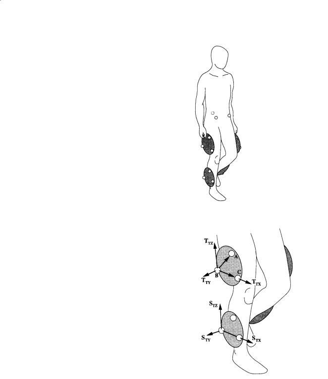
The predominant approach for the collection of clinical gait data involves the placement of external markers on the surface of body segments that are aligned with particular bony landmarks. These markers are commonly attached to the subjects as either discrete units or in rigidly connected clusters (Fig. 8.1). As described briefly above, the products of the data acquisition process are arrays containing the 3-D coordinates (relative to an inertially fixed laboratory coordinate system) of the spatial trajectory of each marker over a gait cycle. If at least three markers or reference points are identified for each body segment, then the six degrees of freedom associated with the position of the segment may be determined. The following example illustrates this straightforward process.

Assume that a cluster of three markers has been attached to the thigh and shank of the test subject as shown in Fig. 8.2. A body-fixed coordinate system may be computed for each cluster. For example, for the thigh, the vector cross product of the unit vectors from markers B to A and B to C produces a vector that is perpendicular to the cluster plane. From these vectors, the unit vectors TTX and TTY may be determined

FIGURE 8.1 Videocamera-based motion measurement systems monitor the displacement of external markers that are placed on the subject’s body segments and aligned with specific bony landmarks. These markers are commonly attached to the subject as either discrete units, e.g., the pelvis, or in rigidly connected clusters, e.g., on the thigh and shank.

FIGURE 8.2 A body-fixed coordinate system may be computed for each cluster of three or more markers. On the thigh, for example, the vector cross product of the unit vectors from markers B to A and B to C produces a vector that is perpendicular to the cluster plane. From these vectors, the unit vectors TTX and TTY may be determined and used to compute the third orthogonal coordinate direction TTZ .

and used to compute the third orthogonal coordinate direction TTZ. In a similar manner the marker-based, or technical, coordinate system may be calculated for the shank, i.e., STX, STY, and STZ. At this point, one might use these two technical coordinate systems to provide an estimate of the absolute orientation of the thigh or shank or the relative angles between the thigh and shank. This assumes that the technical coordinate systems reasonably approximate the anatomical axes of the body segments, e.g., that TTZ approximates the long axis of the thigh. A more rigorous approach incorporates the use of a subject calibration procedure to relate technical coordinate systems with pertinent anatomical directions [Cappozzo, 1984].

136 Biomechanics: Principles and Applications

In a subject calibration, usually performed with the subject standing, additional data are collected by the measurement system that connects the technical coordinate systems to the underlying anatomical structure. For example, as shown in Fig. 8.3, the medial and lateral femoral condyles and the medial and lateral malleoli may be used as anatomical references with the application of additional markers. With the hip center location estimated from markers placed on the pelvis [Bell et al., 1989], and knee and ankle center locations based on the additional markers, anatomical coordinate systems may be computed, e.g., {TA} and {SA}. The relationship between the respective anatomical and technical coordinate system pairs as well as the location of the joint centers in terms of the appropriate technical coordinate system may be stored, to be recalled in the reduction of each frame of the walking data. In this way, the technical coordinate systems (shown in Fig. 8.3) are transformed into alignment with the anatomical coordinate systems.

Once anatomically aligned body-fixed coordinate systems have been computed for each body segment under investigation, one may compute the angular position of the joints and segments in a number of ways. The classical approach of Euler angles is commonly used in clinical gait analysis to describe the motion of the thigh relative to the pelvis (or hip angles), the motion of the shank relative to the thigh (or knee angles), the motion of the foot relative to the shank (or ankle angles), as well as the absolute orientation of the

~

pelvis and foot in space [Grood and Suntay, 1983; Ounpuu et al., 1991]. The joint rotation sequence commonly used for the Euler angle computation is flexion–extension, adduction–abduction, and transverse plane rotation. Alternatively, joint motion has been described through the use of helical axes [Woltring et al., 1985].

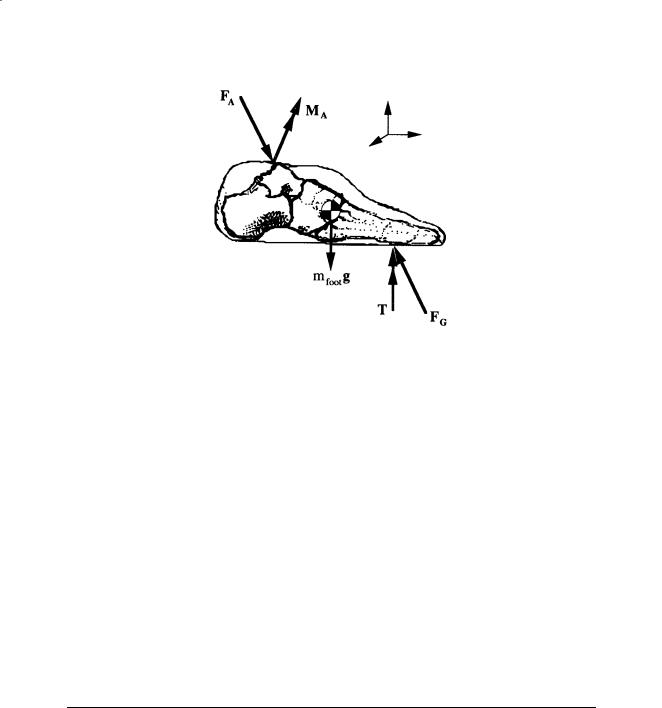
The moments that soft tissue (e.g., muscle, ligaments, joint capsule) forces produce about approximate joint centers may be computed through the use of inverse dynamics, i.e., Newtonian mechanics. For example, the free-body diagram of the foot shown in Fig. 8.4 shows the various external loads to the foot as well as the reactions produced at the ankle. The mass, mass moments of inertia, and location of the center of mass may be estimated from regression-based anthropometric relationships [Dempster et al., 1959], and linear and angular velocity and acceleration may be determined by numerical differentiation. If the ground reaction loads, FG and T, are provided by a force platform, then the unknown ankle reaction force FA may be solved for with Newton’s second law. Euler’s equations of motion may then be applied to compute the net ankle reaction moment, MA. In the application of Euler’s equations of motion, care must be taken to perform the vector operations with all vectors transformed into the foot coordinate system which has been chosen to approximate the principle axes and located at the center of mass of the foot [Greenwood, 1965]. This process may then be repeated for the shank and thigh by using distal joint loads to solve for the proximal joint reactions. The mechanical power associated with a joint moment and the corresponding joint angular velocity may be computed from the vector dot product of the two vectors, e.g., ankle power is computed through MA · ωA where ωA is the angular velocity of the foot relative to the shank.

Although commonly referred to as muscle moments, these net joint reaction moments are generated by several mechanisms, e.g., ligamentous forces, passive muscle and tendon force, and active muscle contractile force, in response to external loads. Currently, clinical muscle force evaluation is not possible because of the scarcity of data related to location of the instantaneous line of muscle force as well as the

FIGURE 8.4 The moments that soft-tissue forces produce about approximate joint centers may be computed through the use of Newtonian mechanics. This free-body diagram of the foot illustrates the external loads to the

foot, e.g., the ground reaction loads, FG and T, and the weight of the foot, mfootg , as well as the unknown reactions produced at the ankle, FA and MA.

overall indeterminacy of the problem. The possibility of the cocontraction of opposing muscle groups also impacts the estimation of bone-on-bone force values, i.e., the magnitude of FA found above reflects the minimum estimated value of the bone-on-bone force at the ankle.

With respect to the kinematic data reduction, the body segments are assumed to be rigid, e.g., softtissue movement relative to underlying bony structures is small. Consequently, marker of instrumentation attachment sites must be selected carefully, e.g., over tendonous structures of the distal shank as opposed to the more proximal muscle masses of the gastrocnemius and soleus. The models described above also assume that the joint center locations remain fixed relative to the respective segmental coordinate systems, e.g., the knee center is fixed relative to the thigh coordinate system. The measurement technology and associated protocols cannot currently produce data of sufficient quality for the reliable determination of instantaneous centers of rotation.

The addition assumptions associated with the gait kinetics model described above are related to the inertial properties of the body segments. Body segment mass and mass distribution, i.e., mass moments of inertia, are generally estimated from statistical relationships derived from cadaver studies. Differences between body types are not typically incorporated into these anthropometric models. Moreover, the mass distribution changes are assumed to be negligible during motion.

8.3 Illustrative Clinical Case

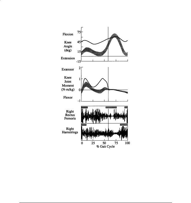
As indicated above, the information available for clinical gait interpretation may include static physical examination measures, stride and temporal data, segment and joint kinematics, joint kinetics, electromyograms, and a video record. With this information the clinical team can assess the patient’s gait deviations, attempt to identify the etiology of the abnormalities, and recommend treatment alternatives. In this way, clinicians are able to isolate the biomechanical insufficiency that may produce a locomotive impairment and require a compensatory response from the patient. For example, a patient may excessively elevate a hip (compensatory) in order to gain additional foot clearance in swing which is perhaps inadequate due to a weak ankle dorsiflexor (primary problem). The knee kinematics and moments and associated electromyographic data shown in Fig. 8.5 were generated by an 11-year-old male with a diagnosis of cerebral palsy, spastic diplegia. Based on the limited knee range of motion, insufficient knee flexion in the swing phase of the gait cycle, and abnormal activity of the rectus femoris in the swing

FIGURE 8.5 These are the knee kinematics and moments and associated electromyographic data for a representative subject with a diagnosis of cerebral palsy, spastic diplegia (including shaded bands/bars indicating one standard deviation about normal).

phase, a transfer of the distal end of the rectus femoris to the sartorius was recommended. Moreover, the excessive knee flexion at initial contact and throughout the stance phase due to overactivity of the hamstrings suggested intramuscular lengthenings of the medial and lateral hamstrings. Transverse plane deviations apparent from the gait analysis (not shown) led to recommendations of derotational osteotomies of both the subject’s femurs and tibias.

8.4 Gait Analysis: Current Status

As indicated in the modeling discussion above, the utility of gait analysis information may be limited by sources of error such as soft tissue displacement relative to bone, estimates of joint center locations, particularly the hip, approximations of the inertial properties of the body segments, and the numerical differentiation of noisy displacement data. Other errors associated with data collection alter the results as well, for example, a marker is improperly placed or a force platform is inadvertently contacted by the swing limb. The evaluation of small subjects weakens the data because intermarker distances are reduced, thereby reducing the precision of angular computations. It is essential that the potential adverse effects of these errors on the gait information be understood and appreciated by the clinician in the interpretation process.

Controversies related to gait analysis techniques include the use of individually placed markers vs. clusters of markers, the estimation of quasi-static, body-fixed locations of joint centers (as described

above) vs. the dynamic determination of the instantaneous locations, and the application of helical or screw axes vs. the use of Euler angles. Additional research and development are needed to resolve these fundamental methodological issues.

Despite these limitations, gait analysis facilitates the systematic quantitative documentation of walking patterns. With the various gait data, the clinician has the opportunity to separate the primary causes of a gait abnormality from compensatory gait mechanisms. Apparent contradictions between the different types of gait information can result in a more carefully developed understanding of the gait deviations. It provides the clinical user the capability to more precisely (than observational gait analysis alone) plan complex multilevel surgeries and evaluate the efficacy of different surgical approaches or orthotic designs. Through gait analysis, movement in planes of motion not easily observed, such as about the long axes of the lower limb segments, may be quantified. Finally, quantities that cannot be observed may be assessed, e.g., muscular activity and joint kinetics. In the future, it is anticipated that our understanding of gait will be enhanced through the application of pattern recognition strategies, coupled dynamics, and the linkage of empirical results derived through inverse dynamics with the simulations provided by forward dynamics modeling.

References

Bell AL, Pederson DR, Brand RA. 1989. Prediction of hip joint center location from external landmarks.

Human Movement Sci 8:3.

Brand RA, Crowninshield RD. 1981. Comment on criteria for patient evaluation tools. J Biomech 14:655. Cappozzo A. 1984. Gait analysis methodology. Human Movement Sci 3:27.

Dempster WT, Gabel WC, Felts WJL. 1959. The anthropometry of manual work space for the seated subjects. Am J Phys Anthropometry 17:289.

Greenwood DT. 1965. Principles of Dynamics, Englewood Cliffs, NJ, Prentice-Hall.

Grood ES, Suntay WJ. 1983. A joint coordinate system for the clinical description of three-dimensional motions: application to the knee. J Biomech Eng 105(2):136.

Õunpuu S, Gage JR, Davis RB. 1991. Three-dimensional lower extremity joint kinetics in normal pediatric gait. J Pediatr Orthop 11:341.

Woltring HJ, Huskies R, DeLange A. 1985. Finite centroid and helical axis estimation from noisy landmark measurement in the study of human joint kinematics. J Biomech 18:379.

Further Information on Gait Analysis Techniques

Allard P, Stokes IAF, Blanchi JP (Eds.) 1995. Three-Dimensional Analysis of Human Movement. Champaign, IL, Human Kinetics.

Berme N, Cappozzo A (Eds.) 1990. Biomechanics of Human Movement: Applications in Rehabilitation, Sports and Ergonomics. Worthington, OH, Bertec Corporation.

Harris GF, Smith PA (Eds.) 1996. Human Motion Analysis. Piscataway, NJ, IEEE Press. Whittle M. 1991. Gait Analysis: An Introduction. Oxford, Butterworth-Heinemann.

Winter DA. 1990. Biomechanics and Motor Control of Human Movement. New York, John Wiley & Sons.

Further Information on Normal and Pathological Gait

Gage JR. 1991. Gait Analysis in Cerebral Palsy. London, MacKeith Press.

Perry J. 1992. Gait Analysis: Normal and Pathological Function. Thorofare, NJ, Slack.

Sutherland DH, Olshen RA, Biden EN et al. 1988. The Development of Mature Walking. London, MacKeith Press.