

Biomechanics Principles and Applications - Schneck and Bronzino
.pdf32 |
Biomechanics: Principles and Applications |
Care must be taken to formulate expressions that will lead to stresses that behave properly. For this reason it is convenient to formulate the strain energy density in terms of the Lagrangian strains:
ei = 1 2(λ2i −1) |
(2.45) |
and in this case we can consider polynomials of the lagrangian strains, qn(er, eθ, ez). Vaishnav et al. [15] proposed using a polynomial of the form:
n |
i |
|
W * = ∑ ∑ai j −i eθi− jezj |
(2.46) |
|
i = 2 |
j = 0 |
|
to approximate the behavior of the canine aorta. They found better correlation with order-three polynomials over order-two, but order-four polynomials did not warrant the additional work.
Later, Fung et al. [10] found very good correlation with an expression of the form:
2 |
[ |
|
] |
|
|
W = |
C |
exp a1(eθ2 |
− ez*2 )+ a2 (ez2 − ez*2 )+ 2a4 (eθez |
− eθ*ez* ) |
(2.47) |
|
|||||
for the canine carotid artery, where e* and e* are the strains in a reference configuration at in situ length
θ z
and pressure. Why should this work? One answer appears to be related to residual stresses and strains. When residual stresses are ignored, large-deformation analysis of thick-walled blood vessels predicts steep distributions in σθ and σz through the vessel wall, with the highest stresses at the interior. This prediction is considered significant because high tensions in the inner wall could inhibit vascularization
and oxygen transport to vascular tissue.
When residual stresses are considered, the stress distributions flatten considerably and become almost uniform at in situ length and pressure. Figure 2.10 shows the radial stress distributions computed for a vessel with β = 1 and β = 1.11. Takamizawa and Hayashi have even considered the case where the strain distribution is uniform in situ [13]. The physiologic implications are that vascular tissue is in a constant
FIGURE 2.10 Stress distributions through the wall at various pressures for the orthotropic vessel.

Mechanics of Blood Vessels |
33 |
state of flux. New tissue is synthesized in a state of stress that allows it to redistribute the internal loads more uniformly. There probably is no stress-free reference state [8, 11, 12]. Continuous dissection of the tissue into smaller and smaller pieces would continue to relieve residual stresses and strains [14].
References
1.Bergel DH. 1961. The static elastic properties of the arterial wall. J Physiol 156:445.
2.Carew TE, Vaishnav RN, Patel DJ. 1968. Compressibility of the arterial walls. Circ Res 23:61.
3.Chu BM, Oka S. 1973. Influence of longitudinal tethering on the tension in thick-walled blood vessels in equilibrium. Biorheology 10:517.
4.Choung CJ, Fung YC. 1986. On residual stresses in arteries. J Biomed Eng 108:189.
5.Dobrin PB. 1978. Mechanical properties of arteries. Physiol Rev 58:397.
6.Dobrin PB, Canfield TR. 1984. Elastase, collagenase, and the biaxial elastic properties of dog carotid artery. Am J Physiol 2547:H124.
7.Dobrin PB, Rovick AA. 1969. Influence of vascular smooth muscle on contractile mechanics and elasticity of arteries. Am J Physiol 217:1644.
8.Dobrin PD, Canfield T, Sinha S. 1975. Development of longitudinal retraction of carotid arteries in neonatal dogs. Experientia 31:1295.
9.Doyle JM, Dobrin PB. 1971. Finite deformation of the relaxed and contracted dog carotid artery.
Microvasc Res 3:400.
10.Fung YC, Fronek K, Patitucci P. 1979. Pseudoelasticity of arteries and the choice of its mathematical expression. Am J Physiol 237:H620.
11.Fung YC, Liu SQ, Zhou JB. 1993. Remodeling of the constitutive equation while a blood vessel remodels itself under strain. J Biomech Eng 115:453.
12.Rachev A, Greenwald S, Kane T, Moore J, Meister J-J. 1994. Effects of age-related changes in the residual strains on the stress distribution in the arterial wall. In J Vossoughi (Ed.), Proceedings of the Thirteenth Society of Biomedical Engineering Recent Developments, pp. 409–412, Washington, D.C., University of District of Columbia.
13.Takamizawa K, Hayashi K. 1987. Strain energy density function and the uniform strain hypothesis for arterial mechanics. J Biomech 20:7.
14.Vassoughi J. 1992. Longitudinal residual strain in arteries. Proc of the 11th South Biomed Engrg Conf, Memphis, TN.
15.Vaishnav RN, Young JT, Janicki JS, Patel DJ. 1972. Nonlinear anisotropic elastic properties of the canine aorta. Biophys J 12:1008.
16.Vaishnav RN, Vassoughi J. 1983. Estimation of residual stresses in aortic segments. In CW Hall (Ed.), Biomedical Engineering, II, Recent Developments, pp. 330–333, New York, Pergamon Press.
17.Von Maltzahn W-W, Desdo D, Wiemier W. 1981. Elastic properties of arteries: a nonlinear twolayer cylindrical model. J Biomech 4:389.
18.Wolinsky H, Glagov S. 1969. Comparison of abdominal and thoracic aortic media structure in mammals. Circ Res 25:677.


Kenton R. Kaufman
Biomechanics Laboratory,
The Mayo Clinic
Kai-Nan An
Biomechanics Laboratory,
The Mayo Clinic
3
Joint-Articulating Surface Motion
3.1 |
Ankle...................................................................................... |
|
|
36 |
|
Geometry of the Articulating Surfaces |
• |
Joint Contact |
• |
|
Axes of Rotation |
|
|
|
3.2 |
Knee....................................................................................... |
|
|
37 |
|
Geometry of the Articulating Surfaces |
• |
Joint Contact |
• |
|
Axes of Rotation |
|
|
|
3.3 |
Hip......................................................................................... |
|
|
40 |
|
Geometry of the Articulating Surfaces |
• |
Joint Contact |
• |
|
Axes of Rotation |
|
|
|
3.4 |
Shoulder ................................................................................ |
|
|
46 |
|
Geometry of the Articulating Surfaces |
• |
Joint Contact |
• |
|
Axes of Rotation |
|
|
|
3.5 |
Elbow..................................................................................... |
|
|
54 |
|
Geometry of the Articulating Surfaces |
• |
Joint Contact |
• |
|
Axes of Rotation |
|
|
|
3.6 |
Wrist ...................................................................................... |
|
|
57 |
|
Geometry of the Articulating Surfaces |
• |
Joint Contact |
• |
|
Axes of Rotation |
|
|
|
3.7 |
Hand...................................................................................... |
|
|
61 |
|
Geometry of the Articulating Surfaces |
• |
Joint Contact |
• |
|
Axes of Rotation |
|
|
|
3.8 |
Summary............................................................................... |
|
|
65 |
Knowledge of joint-articulating surface motion is essential for design of prosthetic devices to restore function; assessment of joint wear, stability, and degeneration; and determination of proper diagnosis and surgical treatment of joint disease. In general, kinematic analysis of human movement can be arranged into two separate categories: (1) gross movement of the limb segments interconnected by joints, or (2) detailed analysis of joint articulating surface motion which is described in this chapter. Gross movement is the relative three-dimensional joint rotation as described by adopting the Eulerian angle system. Movement of this type is described in Chapter 8: Analysis of Gait. In general, the threedimensional unconstrained rotation and translation of an articulating joint can be described utilizing the concept of the screw displacement axis. The most commonly used analytic method for the description of 6-degree-of-freedom displacement of a rigid body is the screw displacement axis [Kinzel et al. 1972; Spoor and Veldpaus, 1980; Woltring et al. 1985].
Various degrees of simplification have been used for kinematic modeling of joints. A hinged joint is the simplest and most common model used to simulate an anatomic joint in planar motion about a single axis embedded in the fixed segment. Experimental methods have been developed for determination
0-8493-1492-5/03/$0.00+$.50 © 2003 by CRC Press LLC
36 |
Biomechanics: Principles and Applications |
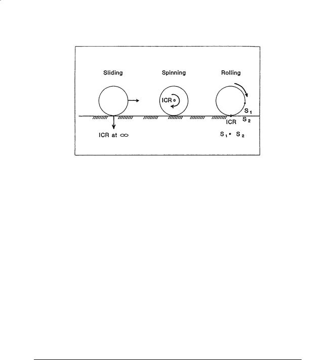
FIGURE 3.1 Three types of articulating surface motion in human joints.
of the instantaneous center of rotation for planar motion. The instantaneous center of rotation is defined as the point of zero velocity. For a true hinged motion, the instantaneous center of rotation will be a fixed point throughout the movement. Otherwise, loci of the instantaneous center of rotation or centrodes will exist. The center of curvature has also been used to define joint anatomy. The center of curvature is defined as the geometric center of coordinates of the articulating surface.
For more general planar motion of an articulating surface, the term sliding, rolling, and spinning are commonly used (Fig. 3.1). Sliding (gliding) motion is defined as the pure translation of a moving segment against the surface of a fixed segment. The contact point of the moving segment does not change, while the contact point of the fixed segment has a constantly changing contact point. If the surface of the fixed segment is flat, the instantaneous center of rotation is located at infinity. Otherwise, it is located at the center of curvature of the fixed surface. Spinning motion (rotation) is the exact opposite of sliding motion. In this case, the moving segment rotates, and the contact points on the fixed surface does not change. The instantaneous center of rotation is located at the center of curvature of the spinning body that is undergoing pure rotation. Rolling motion occurs between moving and fixed segments where the contact points in each surface are constantly changing and the arc lengths of contact are equal on each segment. The instantaneous center of rolling motion is located at the contact point. Most planar motion of anatomic joints can be described by using any two of these three basic descriptions.
In this chapter, various aspects of joint-articulating motion are covered. Topics include the anatomical characteristics, joint contact, and axes of rotation. Joints of both the upper and lower extremity are discussed.
3.1 Ankle
The ankle joint is composed of two joints: the talocrural (ankle) joint and the talocalcaneal (subtalar joint). The talocrural joint is formed by the articulation of the distal tibia and fibula with the trochlea of the talus. The talocalcaneal joint is formed by the articulation of the talus with the calcaneus.
Geometry of the Articulating Surfaces
The upper articular surface of the talus is wedge-shaped, its width diminishing from front to back. The talus can be represented by a conical surface. The wedge shape of the talus is about 25% wider in front than behind with an average difference of 2.4 mm ± 1.3 mm and a maximal difference of 6 mm [Inman, 1976].

Joint-Articulating Surface Motion |
|
|
|
37 |
||
|
TABLE 3.1 Talocalcaneal (Ankle) Joint Contact Area |
|
|
|||
|
|
|
|
|
|
|
|
Investigators |
Plantarflexion |
Neutral |
Dorsiflexion |
||
|
|
|
|
|
|
|
|
Ramsey and Hamilton [1976] |
|
|
4.40 ± 1.21 |
|
|
|
Kimizuka et al. [1980] |
|
|
4.83 |
|
|
|
Libotte et al. [1982] |
5.01 |
(30°) |
5.41 |
3.60 (30°) |
|
|
Paar et al. [1983] |
4.15 |
(10°) |
4.15 |
3.63 (10°) |
|
|
Macko et al. [1991] |
3.81 |
± 0.93 (15°) |
5.2 ± 0.94 |
5.40 ± 0.74 (10°) |
|
|
Driscoll et al. [1994] |
2.70 |
± 0.41 (20°) |
3.27 ± 0.32 |
2.84 ± 0.43 (20°) |
|
|
Hartford et al. [1995] |
|
|
3.37 ± 0.52 |
|
|
|
Pereira et al. [1996] |
1.49 |
(20°) |
1.67 |
1.47 (10°) |
|
|
|
|
|
|
|
|
Note: The contact area is expressed in square centimeters.
Joint Contact
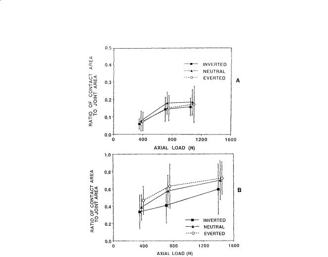
The talocrural joint contact area varies with flexion of the ankle (Table 3.1). During plantarflexion, such as would occur during the early stance phase of gait, the contact area is limited and the joint is incongruous. As the position of the joint progresses from neutral to dorsiflexion, as would occur during the midstance of gait, the contact area increases and the joint becomes more stable. The area of the subtalar articulation is smaller than that of the talocrural joint. The contact area of the subtalar joint is 0.89 ± 0.21 cm2 for the posterior facet and 0.28 ± 15 cm2 for the anterior and middle facets [Wang et al., 1994]. The total contact area (1.18 ± 0.35 cm2) is only 12.7% of the whole subtalar articulation area (9.31 ± 0.66 cm2) [Wang et al., 1994]. The contact area/joint area ratio increases with increases in applied load (Fig. 3.2).
Axes of Rotation
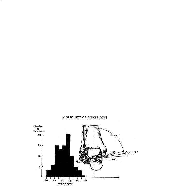
Joint motion of the talocrural joint has been studied to define the axes of rotation and their location with respect to specific anatomic landmarks (Table 3.2). The axis of motion of the talocrural joint essentially passes through the inferior tibia at the fibular and tibial malleoli (Fig. 3.3). Three types of motion have been used to describe the axes of rotation: fixed, quasi-instantaneous, and instantaneous axes. The motion that occurs in the ankle joints consists of dorsiflexion and plantarflexion. Minimal or no transverse rotation takes place within the talocrural joint. The motion in the talocrural joint is intimately related to the motion in the talocalcaneal joint which is described next.
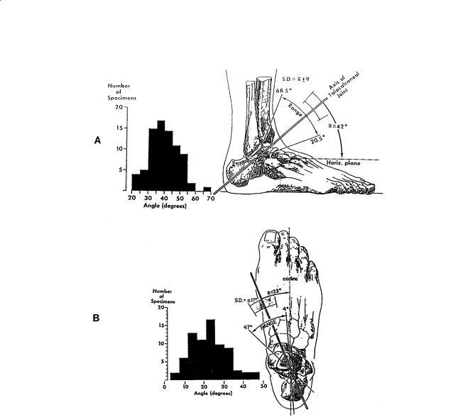
The motion axes of the talocalcaneal joint have been described by several authors (Table 3.3). The axis of motion in the talocalcaneal joint passes from the anterior medial superior aspect of the navicular bone to the posterior lateral inferior aspect of the calcaneus (Fig. 3.4). The motion that occurs in the talocalcaneal joint consists of inversion and eversion.
3.2 Knee
The knee is the intermediate joint of the lower limb. It is composed of the distal femur and proximal tibia. It is the largest and most complex joint in the body. The knee joint is composed of the tibiofemoral articulation and the patellofemoral articulation.
Geometry of the Articulating Surfaces
The shape of the articular surfaces of the proximal tibia and distal femur must fulfill the requirement that they move in contact with one another. The profile of the femoral condyles varies with the condyle examined (Fig. 3.5 and Table 3.4). The tibial plateau widths are greater than the corresponding widths of the femoral condyles (Fig. 3.6 and Table 3.5). However, the tibial plateau depths are less than those
38 |
Biomechanics: Principles and Applications |
FIGURE 3.2 Ratio of total contact area to joint area in the (A) anterior/middle facet and (B) posterior facet of the subtalar joint as a function of applied axial load for three different positions of the foot. (Source: Wagner UA, Sangeorzan BJ, Harrington RM, Tencer AF. 1992. Contact characteristics of the subtalar joint: load distribution between the anterior and posterior facets. J Orthop Res 10:535. With permission.)
of the femoral condyle distances. The medial condyle of the tibia is concave superiorly (the center of curvature lies above the tibial surface) with a radius of curvature of 80 mm [Kapandji, 1987]. The lateral condyle is convex superiorly (the center of curvature lies below the tibial surface) with a radius of curvature of 70 mm [Kapandji, 1987]. The shape of the femoral surfaces is complementary to the shape of the tibial plateaus. The shape of the posterior femoral condyles may be approximated by spherical surfaces (Table 3.4).
The geometry of the patellofemoral articular surfaces remains relatively constant as the knee flexes. The knee sulcus angle changes only ±3.4° from 15 to 75° of knee flexion (Fig. 3.7). The mean depth index varies by only ±4% over the same flexion range (Fig. 3.7). Similarly, the medial and lateral patellar facet angles (Fig. 3.8) change by less than a degree throughout the entire knee flexion range (Table 3.6). However, there is a significant difference between the magnitude of the medial and lateral patellar facet angles.
Joint Contact
The mechanism of movement between the femur and tibia is a combination of rolling and gliding. Backward movement of the femur on the tibia during flexion has long been observed in the human knee. The magnitude of the rolling and gliding changes through the range of flexion. The tibial–femoral contact
Joint-Articulating Surface Motion |
39 |
||
TABLE 3.2 Axis of Rotation for the Ankle |
|
||
|
|
|
|
Investigator |
Axisa |
Position |
|
Elftman [1945] |
Fix. |
67.6° ± 7.4° with respect to sagittal plane |
|
Isman and Inman [1969] |
Fix. |
8 mm anterior, 3 mm inferior to the distal tip of the lateral malleolus; 1 mm posterior, |
|
|
|
5 mm inferior to the distal tip of the medial malleolus |
|
Inman and Mann [1979] |
Fix. |
79° (68–88°) with respect to the sagittal plane |
|
Allard et al. [1987] |
Fix. |
95.4° ± 6.6° with respect to the frontal plane, 77.7° ± 12.3° with respect to the sagittal |
|
|
|
plane, and 17.9° ± 4.5° with respect to the transverse plane |
|
Singh et al. [1992] |
Fix. |
3.0 mm anterior, 2.5 mm inferior to distal tip of lateral malleolus, 2.2 mm posterior, |
|
|
|
10 mm inferior to distal tip of medial malleolus |
|
Sammarco et al. [1973] |
Ins. |
Inside and outside the body of the talus |
|
D’Ambrosia et al. [1976] |
Ins. |
No consistent pattern |
|
Parlasca et al. [1979] |
Ins. |
96% within 12 mm of a point 20 mm below the articular surface of the tibia along |
|
|
|
the long axis. |
|
Van Langelaan [1983] |
Ins. |
At an approximate right angle to the longitudinal direction of the foot, passing through |
|
|
|
the corpus tali, with a direction from anterolaterosuperior to posteromedioinferior |
|
Barnett and Napier [1952] |
Q-I |
Dorsiflexion: down and lateral |
|
|
|
Plantarflexion: down and medial |
|
Hicks [1953] |
Q-I |
Dorsiflexion: 5 mm inferior to tip of lateral malleolus to 15 mm anterior to tip of |
|
|
|
medial malleolus |
|
|
|
Plantarflexion: 5 mm superior to tip of lateral malleolus to 15 mm anterior, 10 mm |
|
|
|
inferior to tip of medial malleolus |
|
|
|
|
|
a Fix. = fixed axis of rotation; Ins. = instantaneous axis of rotation; Q-I = quasi-instantaneous axis of rotation
FIGURE 3.3 Variations in angle between middle of tibia and empirical axis of ankle. The histogram reveals a considerable spread of individual values. (Source: Inman VT. 1976. The Joints of the Ankle, Baltimore, Williams & Wilkins. With permission.)
point has been shown to move posteriorly as the knee is flexed, reflecting the coupling of anterior/ posterior motion with flexion/extension (Fig. 3.9). During flexion, the weight-bearing surfaces move backward on the tibial plateaus and become progressively smaller (Table 3.7).
It has been shown that in an intact knee at full extension the center of pressure is approximately 25 mm from the anterior edge of the knee joint line [Andriacchi et al., 1986]. This net contact point moves posteriorly with flexion to approximately 38.5 mm from the anterior edge of the knee joint. Similar displacements have been noted in other studies (Table 3.8).

40 |
|
Biomechanics: Principles and Applications |
TABLE 3.3 Axis of Rotation for the Talocalcaneal (Subtalar) Joint |
||
|
|
|
Investigator |
Axisa |
Position |
Manter [1941] |
Fix. |
16° (8–24°) with respect to sagittal plane, and 42° (29–47°) with respect to transverse |
|
|
plane |
Shephard [1951] |
Fix. |
Tuberosity of the calcaneus to the neck of the talus |
Hicks [1953] |
Fix. |
Posterolateral corner of the heel to superomedial aspect of the neck of the talus |
Root et al. [1966] |
Fix. |
17° (8–29°) with respect to sagittal plane, and 41° (22–55°) with respect to transverse |
|
|
plane |
Isman and Inman [1969] |
Fix. |
23° ± 11° with respect to sagittal plane, and 41° ± 9° with respect to transverse plane |
Kirby [1947] |
Fix. |
Extends from the posterolateral heel, posteriorly, to the first intermetatarsal space, |
|
|
anteriorly |
Rastegar et al. [1980] |
Ins. |
Instant centers of rotation pathways in posterolateral quadrant of the distal |
|
|
articulating tibial surface, varying with applied load |
Van Langelaan [1983] |
Ins. |
A bundle of axes that make an acute angle with the longitudinal direction of the foot |
|
|
passing through the tarsal canal having a direction from anteromediosuperior to |
|
|
posterolateroinferior |
Engsberg [1987] |
Ins. |
A bundle of axes with a direction from anteromediosuperior to posterolateroinferior |
|
|
|
a Fix. = fixed axis of rotation; Ins. = instantaneous axis of rotation
The patellofemoral contact area is smaller than the tibiofemoral contact area (Table 3.9). As the knee joint moves from extension to flexion, a band of contact moves upward over the patellar surface (Fig. 3.10). As knee flexion increases, not only does the contact area move superiorly, but it also becomes larger. At 90° of knee flexion, the contact area has reached the upper level of the patella. As the knee continues to flex, the contact area is divided into separate medial and lateral zones.
Axes of Rotation
The tibiofemoral joint is mainly a joint with two degrees of freedom. The first degree of freedom allows movements of flexion and extension in the sagittal plane. The axis of rotation lies perpendicular to the sagittal plane and intersects the femoral condyles. Both fixed axes and screw axes have been calculated (Fig. 3.11). In Fig. 3.11, the optimal axes are fixed axes, whereas the screw axis is an instantaneous axis. The symmetric optimal axis is constrained such that the axis is the same for both the right and left knee. The screw axis may sometimes coincide with the optimal axis but not always, depending upon the motions of the knee joint. The second degree of freedom is the axial rotation around the long axis of the tibia. Rotation of the leg around its long axis can only be performed with the knee flexed. There is also an automatic axial rotation which is involuntarily linked to flexion and extension. When the knee is flexed, the tibia internally rotates. Conversely, when the knee is extended, the tibia externally rotates.
During knee flexion, the patella makes a rolling/gliding motion along the femoral articulating surface. Throughout the entire flexion range, the gliding motion is clockwise (Fig. 3.12). In contrast, the direction of the rolling motion is counter-clockwise between 0° and 90° and clockwise between 90° and 120° (Fig. 3.12). The mean amount of patellar gliding for all knees is approximately 6.5 mm per 10° of flexion between 0° and 80° and 4.5 mm per 10° of flexion between 80° and 120°. The relationship between the angle of flexion and the mean rolling/gliding ratio for all knees is shown in Fig. 3.13. Between 80° and 90° of knee flexion, the rolling motion of the articulating surface comes to a standstill and then changes direction. The reversal in movement occurs at the flexion angle where the quadriceps tendon first contacts the femoral groove.
3.3 Hip
The hip joint is composed of the head of the femur and the acetabulum of the pelvis. The hip joint is one of the most stable joints in the body. The stability is provided by the rigid ball-and-socket configuration.
Joint-Articulating Surface Motion |
41 |
FIGURE 3.4 (A) Variations in inclination of axis of subtalar joint as projected upon the sagittal plane. The distribution of the measurements on the individual specimens is shown in the histogram. The single observation of an angle of almost 70° was present in a markedly cavus foot. (B) Variations in position of subtalar axis as projected onto the transverse plane. The angle was measured between the axis and the midline of the foot. The extent of individual variation is shown on the sketch and revealed in the histogram. (Source: Inman VT. 1976. The Joints of the Ankle, Baltimore, Williams & Wilkins. With permission.)
Geometry of the Articulating Surfaces
The femoral head is spherical in its articular portion which forms two-thirds of a sphere. The diameter of the femoral head is smaller for females than for males (Table 3.10). In the normal hip, the center of the femoral head coincides exactly with the center of the acetabulum. The rounded part of the femoral head is spheroidal rather than spherical because the uppermost part is flattened slightly. This causes the load to be distributed in a ringlike pattern around the superior pole. The geometrical center of the femoral head is traversed by the three axes of the joint, the horizontal axis, the vertical axis, and the anterior/posterior axis. The head is supported by the neck of the femur, which joins the shaft. The axis of the femoral neck is obliquely set and runs superiorly, medially, and anteriorly. The angle of inclination of the femoral neck to the shaft in the frontal plane is the neck-shaft angle (Fig. 3.14). In most adults,