Biomechanics Principles and Applications - Schneck and Bronzino

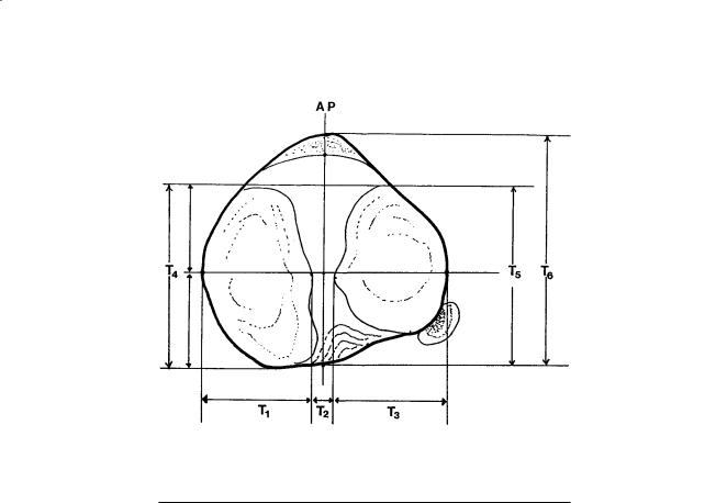
FIGURE 3.5 Geometry of distal femur. The distances are defined in Table 3.4.

TABLE 3.4 Geometry of the Distal Femur

Note: See Fig. 3.5 for location of measurements.

Sources: Yoshioka Y, Siu D, Cooke TDV. 1987. The anatomy of functional axes of the femur. J Bone Joint Surg 69A(6):873–880. Kurosawa H, Walker PS, Abe S, Garg A, Hunter T. 1985. Geometry and motion of the knee for implant and orthotic design. J Biomech 18(7):487.

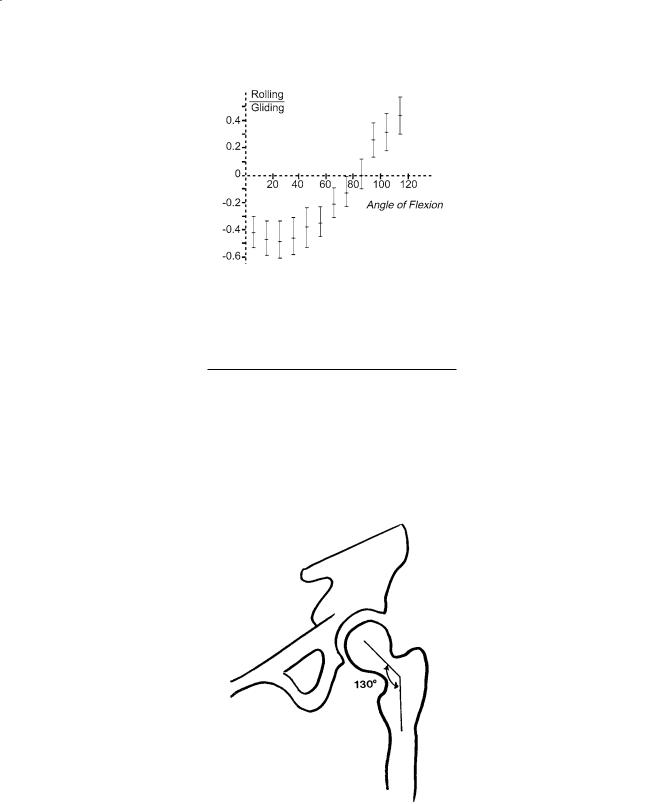
this angle is about 130° (Table 3.10). An angle exceeding 130° is known as coxa valga; an angle less than 130° is known as coxa vara. The femoral neck forms an acute angle with the transverse axis of the femoral condyles. This angle faces medially and anteriorly and is called the angle of anteversion (Fig. 3.15). In the adult, this angle averages about 7.5° (Table 3.10).

The acetabulum receives the femoral head and lies on the lateral aspect of the hip. The acetabulum of the adult is a hemispherical socket. Its cartilage area is approximately 16 cm2 [Von Lanz and Wauchsmuth, 1938]. Together with the labrum, the acetabulum covers slightly more than 50% of the femoral head [Tönnis, 1987]. Only the sides of the acetabulum are lined by articular cartilage, which is interrupted inferiorly by the deep acetabular notch. The central part of the cavity is deeper than the articular cartilage and is nonarticular. This part is called the acetabular fossae and is separated from the interface of the pelvic bone by a thin plate of bone.

FIGURE 3.6 Contour of the tibial plateau (transverse plane). The distances are defined in Table 3.5.

TABLE 3.5 Geometry of the Proximal Tibia

Source: Yoshioka Y, Siu D, Scudamore RA, Cooke TDV. 1989. Tibial anatomy in functional axes. J Orthop Res 7:132.

Joint Contact

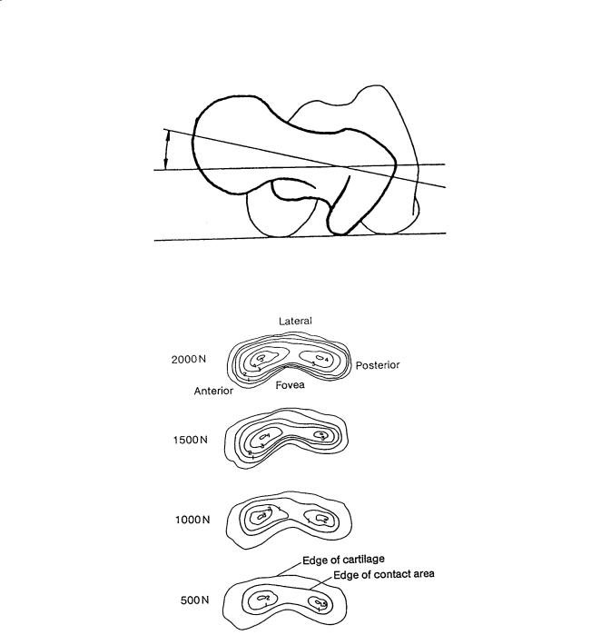
Miyanaga et al. [1984] studied the deformation of the hip joint under loading, the contact area between the articular surfaces, and the contact pressures. They found that at loads up to 1000 N, pressure was distributed largely to the anterior and posterior parts of the lunate surface with very little pressure applied to the central portion of the roof itself. As the load increased, the contact area enlarged to include the outer and inner edges of the lunate surface (Fig. 3.16). However, the highest pressures were still measured anteriorly and posteriorly. Of five hip joints studied, only one had a pressure maximum at the zenith or central part of the acetabulum.

Davy et al. [1989] utilized a telemetered total hip prosthesis to measure forces across the hip after total hip arthroplasty. The orientation of the resultant joint contact force varies over a relatively limited range during the weight-load-bearing portions of gait. Generally, the joint contact force on the ball of the hip prosthesis is located in the anterior/superior region. A three-dimensional plot of the resultant joint force during the gait cycle, with crutches, is shown in Fig. 3.17.

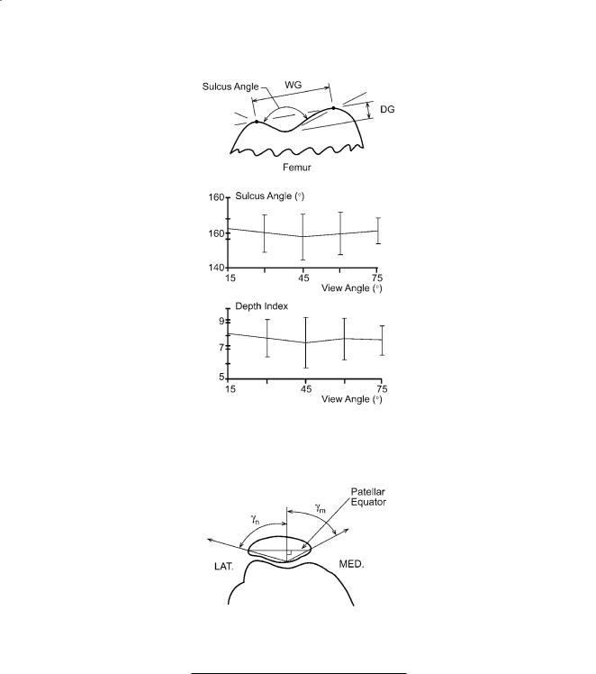
FIGURE 3.7 The trochlear geometry indices. The sulcus angle is the angle formed by the lines drawn from the top of the medial and lateral condyles to the deepest point of the sulcus. The depth index is the ratio of the width of the groove (WG) to the depth (DG). Mean and SD; n = 12. (Source: Farahmand F. et al. 1998. Quantitative study of the quadriceps muscles and trochlear groove geometry related to instability of the patellofemoral joint, J Orthop Res 16(1):140.)

FIGURE 3.8 Medial (γm) and lateral (γn) patellar facet angles. (Source: Ahmed AM, Burke DL, Hyder A. 1987. Force analysis of the patellar mechanism. J Orthop Res 5:69–85.)

TABLE 3.6 Patellar Facet Angles

a SD

Source: Ahmed AM, Burke DL, Hyder A. 1987. Force analysis of the patellar mechanism. J Orthop Res 5:69–85.

FIGURE 3.9 Tibio-femoral contact area as a function of knee flexion angle. (Source: Iseki F, Tomatsu T. 1976. The biomechanics of the knee joint with special reference to the contact area. Keio J Med 25:37. With permission.)

TABLE 3.7 Tibiofemoral Contact Area

Source: Maquet PG, Vandberg AJ, Simonet JC. 1975. Femorotibial weight bearing areas: experimental determination. J Bone Joint Surg 57A(6):766.

TABLE 3.8 Posterior Displacement of the Femur

Relative to the Tibia

Axes of Rotation

The human hip is a modified spherical (ball-and-socket) joint. Thus, the hip possesses three degrees of freedom of motion with three correspondingly arranged, mutually perpendicular axes that intersect at the geometric center of rotation of the spherical head. The transverse axis lies in the frontal plane and controls movements of flexion and extension. An anterior/posterior axis lies in the sagittal plane and controls movements of adduction and abduction. A vertical axis which coincides with the long axis of the limb when the hip joint is in the neutral position controls movements of internal and external rotation. Surface motion in the hip joint can be considered as spinning of the femoral head on the

Source: Hubert HH, Hayes WC. 1984. Patellofemoral contact pressures: the influence of Q-angle and tendofemoral contact. J Bone Joint Surg 66A(5):715–725.

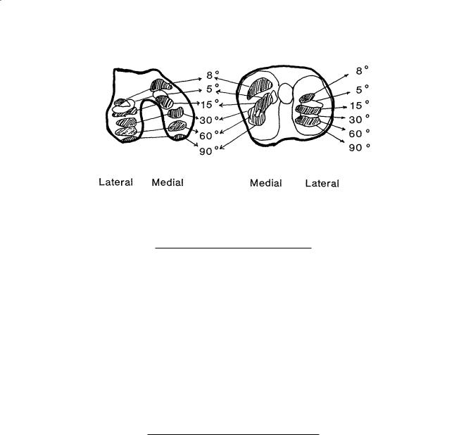
FIGURE 3.10 Diagrammatic representation of patella contact areas for varying degrees of knee flexion. (Source: Goodfellow J, Hungerford DS, Zindel M. 1976. Patellofemoral joint mechanics and pathology. J Bone Joint Surg 58B(3):288.)

acetabulum. The pivoting of the bone socket in three planes around the center of rotation in the femoral head produces the spinning of the joint surfaces.

3.4 Shoulder

The shoulder represents the group of structures connecting the arm to the thorax. The combined movements of four distinct articulations—glenohumeral, acromioclavicular, sternoclavicular, and scapu- lothoracic—allow the arm to be positioned in space.

Geometry of the Articulating Surfaces

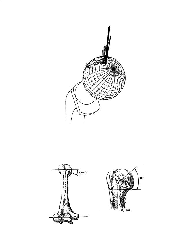
The articular surface of the humerus is approximately one-third of a sphere (Fig. 3.18). The articular surface is oriented with an upward tilt of approximately 45° and is retroverted approximately 30° with respect to the condylar line of the distal humerus [Morrey and An, 1990]. The average radius of curvature of the humeral head in the coronal plane is 24.0 ± 2.1 mm [Iannotti et al., 1992]. The radius of curvature

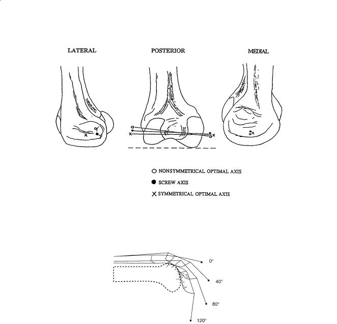
FIGURE 3.11 Approximate location of the optimal axis (case 1—nonsymmetric, case 3—symmetric), and the screw axis (case 2) on the medial and lateral condyles of the femur of a human subject for the range of motion of 0–90° flexion (standing to sitting, respectively). (Source: Lewis JL, Lew WD. 1978. A method for locating an optimal “fixed” axis of rotation for the human knee joint. J Biomech Eng 100:187. With permission.)

FIGURE 3.12 Position of patellar ligament, patella, and quadriceps tendon and location of the contact points as a function of the knee flexion angle. (Source: van Eijden TMGJ, Kouwenhoven E, Verburg J, et al. 1986. A mathematical model of the patellofemoral joint. J Biomech 19(3):227.)

in the anteroposterior and axillary-lateral view is similar, measuring 13.1 ± 1.3 mm and 22.9 ± 2.9 mm, respectively [McPherson et al., 1997]. The humeral articulating surface is spherical in the center. However, the peripheral radius is 2 mm less in the axial plane than in the coronal plane. Thus the peripheral contour of the articular surface is elliptical with a ratio of 0.92 [Iannotti et al., 1992]. The major axis is superior to inferior and the minor axis is anterior to posterior [McPherson et al., 1997]. More recently, the three-dimensional geometry of the proximal humerus has been studied extensively. The articular surface, which is part of a sphere, varies individually in its orientation with respect to inclination and retroversion, and it has variable medial and posterior offsets [Boileau and Walch, 1997]. These findings have great impact in implant design and placement in order to restore soft-tissue function.

The glenoid fossa consists of a small, pear-shaped, cartilage-covered bony depression that measures 39.0 ± 3.5 mm in the superior/inferior direction and 29.0 ± 3.2 mm in the anterior/posterior direction [Iannotti et al., 1992]. The anterior/posterior dimension of the glenoid is pear-shaped with the lower

FIGURE 3.15 The normal anteversion angle formed by a line tangent to the femoral condyles and the femoral neck axis, as displayed in the superior view.

FIGURE 3.16 Pressure distribution and contact area of hip joint. The pressure is distributed largely to the anterior and posterior parts of the lunate surface. As the load increased, the contact area increased. (Source: Miyanaga Y, Fukubayashi T, Kurosawa H. 1984. Contact study of the hip joint: load deformation pattern, contact area, and contact pressure. Arch Orth Trauma Surg 103:13. With permission.)

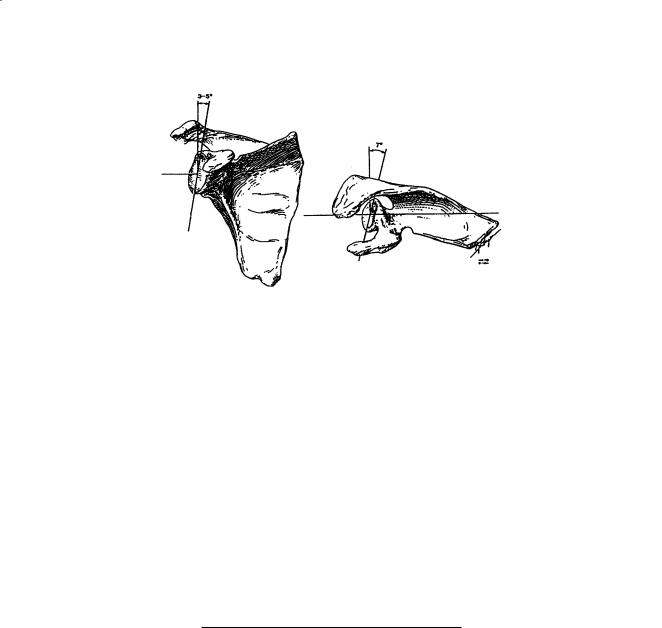
superior to inferior (coronal plane) and relatively flatter in an anterior to posterior direction (sagittal plane). Glenoid depth is 5.0 ± 1.1 mm in the anteroposterior view and 2.9 ± 1.0 mm in the axillarylateral [McPherson et al., 1997], again confirming that the glenoid is more curved superior to inferior. In the coronal plane the articular surface of the glenoid comprises an arc of approximately 75° and in the transverse plane the arc of curvature of the glenoid is about 50° [Morrey and An, 1990]. The glenoid has a slight upward tilt of about 5° [Basmajian and Bazant, 1959] with respect to the medial border of the scapula (Fig. 3.19) and is retroverted a mean of approximately 7° [Saha, 1971]. The relationship of the

FIGURE 3.19 The glenoid faces slightly superior and posterior (retroverted) with respect to the body of the scapula. (By permission of the Mayo Foundation.)

and glenoid in the frontal and axial planes were measured [Jobe and Iannotti, 1995]. In the coronal plane, the humeral heads had an arc of 159° covered by 96° of glenoid, leaving 63° of cartilage uncovered. In the transverse plane, the humeral arc of 160° is opposed by 74° of glenoid, leaving 86° uncovered.

Joint Contact

The degree of conformity and constraint between the humeral head and glenoid has been represented by conformity index (radius of head/radius of glenoid) and constraint index (arc of enclosure/360) [McPherson, 1997]. Based on the study of 93 cadaveric specimens, the mean conformity index was 0.72 in the coronal and 0.63 in the sagittal plane. There was more constraint to the glenoid in the coronal vs. sagittal plane (0.18 vs. 0.13). These anatomic features help prevent superior–inferior translation of the humeral head but allow translation in the sagittal plane. Joint contact areas of the glenohumeral joint tend to be greater at mid-elevation positions than at either of the extremes of joint position (Table 3.11). These results suggest that the glenohumeral surface is maximum at these more functional positions, thus distributing joint load over a larger region in a more stable configuration. The contact point moves

TABLE 3.11 Glenohumeral Contact Areas

Note: SR = starting external rotation which allowed the shoulder to reach maximal elevation in the scapular plane (≈40° ± 8°); NA = not applicable.

Source: Soslowsky LJ, Flatow EL, Bigliani LU, Pablak RJ, Mow VC, Athesian GA. 1992. Quantitation of in situ contact areas at the glenohumeral joint: a biomechanical study. J Orthop Res 10(4):524. With permission.