Table 16.1 Betas for selected firms in two industries
Airline companies
Beta
Food processing companies
Beta
American Airlines
2.52
Campbell Soups
0.44
United Airlines
1.92
H. J. Heinz
0.30
Northwest
1.88
Kraft Foods
0.30
Delta Airlines
1.70
Nabisco
0.28
British Airways
1.70
Kellogg’s
0.03
Source: www.dbc.com, Jan. 29, 2004.
R j
= R f + (Rm - R f )b j
(16.2)
where Rj is the expected rate of return on security j; Rf is the riskless rate of interest; Rm is the expected rate of return on the market portfolio, which is a group of risky securities, such as Standard & Poor’s 500 Stocks or the London Financial Times Stock Exchange 100; and bj is the systematic risk of security j. This equation, known as the security market line, consists of the riskless rate of interest (Rf) and a risk premium [(Rm - Rf)bj]. It is important to understand that beta - bj = [(Rj - Rf)/(Rm - Rf)] – is an index of volatility in the excess return of one security relative to that of a market portfolio.
AGGRESSIVE VERSUS DEFENSIVE STOCKS Because beta reflects the systematic risk of a stock or a mutual fund relative to that of the market as a whole, the market index is assigned a beta of 1. Beta may be used to classify stocks into two broad categories: aggressive and defensive. Aggressive stocks are those stocks that have betas greater than 1. Their returns rise (fall) more than the market index rises (falls). Defensive stocks are those stocks that have betas less than 1. Their returns fluctuate less than the market index. Those stocks with betas equal to 1 are frequently called neutral stocks.
Table 16.1 shows a sample of betas for 10 stocks: five aggressive stocks (airline companies) and five defensive stocks (food processing companies). Food processing companies have very stable earnings streams because their products are necessities. Swings in the earnings and stock returns of food processing companies are modest relative to the earnings and returns of most companies in the economy. Thus, food processing companies have a very low level of systematic risk and low betas.
At the other extreme, airline revenues are closely tied to passenger miles, which are in turn very sensitive to changes in economic activity. This basic variability in revenues is amplified by high operating and financial leverage. These factors cause airline earnings and returns to produce wide variations relative to swings in the earnings and returns of most firms in the economy. Hence, airline companies have high betas.
Is beta one of the best ways to predict how your mutual fund or stock might perform in a market downturn or upturn? Table 16.2 shows average returns for US stock funds during the sharp decline from the peak on July 17, 1998, through August 31, 1998. In this particular downturn caused by the Asian financial crisis, beta has done a pretty good job of predicting which funds would be hit hardest or the least hard. For example, the 25 percent of US stock funds with the highest beta declined 27.68 percent in the period from July 17 through August 31. On the other hand, the 25 percent of US stock funds with the lowest beta lost only 17.77 percent during the same period. In that period, Standard & Poor’s 500 Stocks lost 19.13 percent.
KEY TERMINOLOGY
403
Table 16.2 Average returns for US stock funds from July 17, 1998, to August 31, 1998
Average
Number of funds
Beta
return (%)
in group
Greater than 1.09
-27.68
461
Between 1.08 and 0.99
-20.93
486
Below 0.86
-17.77
434
Source: The Wall Street Journal, Oct. 15, 1998, p. R17.
Return
Security market line
Region of acceptance
Region of rejection
Rf
0
Risk
Figure 16.2 The security market line
In a portfolio context, the security market line constitutes various portfolios that combine a riskless security and a portfolio of risky securities. The general decision rule for accepting a risky project (j), can be stated as follows:
R j > R f + (Rm - R f )b j
(16.3)
This decision rule implies that to accept security j, its expected return must exceed the investor’s hurdle rate, which is the sum of the riskless rate of interest plus a risk premium for the riskiness of the security. Figure 16.2 shows the decision rule in general terms: accept all securities that plot above the security market line and reject all securities that plot below the security market line.
404 INTERNATIONAL PORTFOLIO INVESTMENT
16.1.3Correlation coefficients
The portfolio effect is defined as the extent to which unsystematic risks of individual securities tend to offset each other. The portfolio effect, or portfolio standard deviation, depends not only on the standard deviation of each security but also on the degree of correlation between two or more securities. The correlation coefficient measures the degree of correlation between two securities and varies from zero (no correlation, or independence) to 1.0 (perfect correlation).
A correlation coefficient of -1.0 means that the two sets of returns for two securities tend to move in exactly opposite directions. Assume that a boom occurs. Security A is expected to earn $100, while security B is expected to earn nothing. In contrast, if a recession occurs, security A would earn nothing, whereas security B would earn $100. Consequently, these two securities are perfectly negatively correlated. Diversification can totally eliminate unsystematic risk when two securities are perfectly negatively correlated.
A correlation coefficient of +1.0 means that two sets of returns for two securities tend to move in exactly the same direction. Suppose that a boom occurs. Securities X and Y would earn an equal amount of $200. But if a recession occurs, they would yield an equal amount of $50. Then we can say that these two securities are perfectly positively correlated. In this case, diversification would not reduce unsystematic risk at all.
A correlation coefficient of zero means that the two sets of returns for two securities are uncorrelated or independent of each other. In this scenario, diversification would reduce unsystematic risk considerably.
Because the degree of correlation among securities depends on economic factors, most pairs of domestic securities have a correlation coefficient of between 0 and +1.0. Most stock prices are likely to be high during a boom, while they are likely to be low during a recession. But different product lines and different geographical markets tend to have a relatively low degree of correlation to each other. Thus, international diversification may eliminate unsystematic risk and reduce domestic systematic risk considerably.
16.1.4Portfolio return and risk
Portfolio return is the expected rate of return on a portfolio of securities. The expected portfolio return is simply a weighted average of the expected returns of the securities that make up the portfolio. One way to measure the benefits of international diversification is to consider the expected return and standard deviation of return for a portfolio that consists of US and foreign portfolios. Such a portfolio return may be computed as follows:
R p = X us Rus + XfnR fn
(16.4)
where Rp is the portfolio return, Xus is the percentage of funds invested in the US portfolio, Rus is the expected return on the US portfolio, Xfn is the percentage of funds invested in the foreign portfolio, and Rfn is the expected return on the foreign portfolio.
The standard deviation of a portfolio measures the riskiness of the portfolio. The standard deviation of a two-security portfolio can be calculated as follows:
s p = X us2 sus2 + X 2fn s2fn + 2X us X fn sus , fn sus sfn
(16.5)
KEY TERMINOLOGY
405
where sp is the portfolio standard deviation, sus is the standard deviation of the US portfolio, sfn is the standard deviation of the foreign portfolio, and sus,fn is the correlation coefficient between the returns on the US and foreign portfolios.
Example 16.1
Assume that an international portfolio consisting of a US portfolio and a foreign portfolio calls for a total investment of $10 million. The US portfolio requires an investment of $4 million and the foreign portfolio requires an investment of $6 million. The expected returns are 8 percent on the US portfolio and 12 percent on the foreign portfolio. The standard deviations are 3.17 percent for the US portfolio and 3.17 percent for the foreign portfolio.
Because the percentage of the international portfolio invested in the US portfolio is 40 percent and that of the foreign portfolio is 60 percent, we can use equation 16.4 to compute the return on the international portfolio:
Rp = (0.4)0.08 + (0.6)0.12 = 10.4%
It is important to recognize that the return on the international portfolio is the same regardless of correlation of returns for the US and foreign portfolios. However, the degree of the international portfolio risk varies according to interportfolio or intersecurity return behavior. Intersecurity returns can be perfectly negatively correlated, statistically independent, or perfectly positively correlated.
Case A: perfectly negative correlation
If the US and foreign portfolios are perfectly negatively correlated, their correlation coefficient becomes -1. The return on the international portfolio and its standard deviation (use equation 16.5) are as follows:
Because the standard deviation of US and foreign portfolios are 3.17 percent each, their weighted average is 3.17 percent (0.0317 ¥ 0.40 + 0.0317 ¥ 0.60). Thus, the standard deviation of the international portfolio is only 20 percent of the weighted average of the two individual standard deviations (0.0063/0.0317). If a considerable number of perfectly negatively correlated projects are available, risk can be almost entirely diversified away. However, perfect negative correlation is seldom found in the real world.
406 INTERNATIONAL PORTFOLIO INVESTMENT
Case B: statistical independence
If these two portfolios are statistically independent, the correlation coefficient between the two is 0. The return of the international portfolio and its standard deviation are as follows:
In this case, the standard deviation of the international portfolio is 72 percent of this weighted average (0.0229/0.0317). This means that international diversification can reduce risk significantly if a considerable number of statistically independent securities are available.
Case C: perfectly positive correlation
If the two portfolios are perfectly positively correlated with each other, their correlation coefficient becomes 1. The portfolio return and its standard deviation are as follows:
The standard deviation of the international portfolio equals the weighted average of the two individual standard deviations. Thus, if all alternative investments are perfectly positively correlated, diversification would not reduce risk at all.
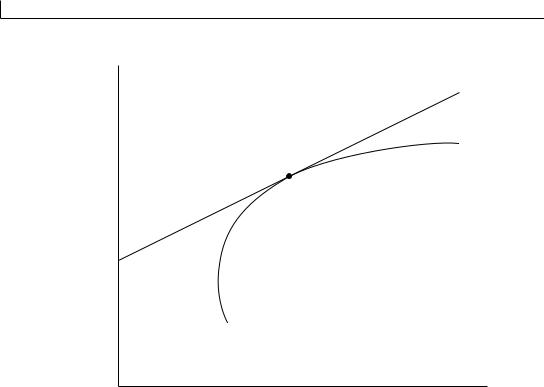
16.1.5The efficient frontier
An efficient portfolio is a portfolio that incurs the smallest risk for a given level of return and/or provides the highest rate of return for a given level of risk. Suppose that A, B, and C are three exclusive portfolios that require the same amount of investment, say, $10 million. They have an equal rate of return, but their respective standard deviations are different. Figure 16.3 shows that A incurs the smallest risk for a given level of return; A is called the efficient portfolio. By the same token, assume that W, X, and Y are three exclusive portfolios that require the same amount of money, say, $10 million. They have the same amount of risk, but their rates of return are different. As shown in figure 16.3, we notice that W provides the highest rate of return for a given level of risk; W is also called the efficient portfolio. If we compute more points such as A and W, we may obtain curve AW by connecting such points. This curve is known as the efficient frontier. Portfolios B, C, X, and Y are inefficient because some other portfolios could give either a lower risk for the same rate of return or a higher return for the same degree of risk.
There are numerous efficient portfolios along the efficient frontier. An efficient frontier does not tell us which portfolio to select, but shows a collection of portfolios that minimize risk for any expected return or that maximize the expected return for any degree of risk. The objective
THE BENEFITS OF INTERNATIONAL DIVERSIFICATION
407
Return
W
X
Y
A B C
0
Risk
Figure 16.3 An efficient frontier
of the investor is to choose the optimal portfolio among those on the efficient frontier. Thus the efficient frontier is necessary but not sufficient for selecting the optimal portfolio. Given an efficient frontier, the choice of the optimal portfolio depends on the security market line.
If investors want to select the optimal portfolio from portfolios on a particular efficient frontier, they should land on the highest security market line. This optimal portfolio is found at the tangency point between the efficient frontier and the security market line. Tangency point M in figure 16.4 marks the highest security market line that investors can obtain with funds available for investment. An optimum portfolio is the portfolio that has, among all possible portfolios, the largest ratio of expected return to risk. Once investors identify the optimal portfolio, they will allocate funds between risky assets and risk-free assets to achieve a desired combination of risk and return.
16.2The Benefits of International Diversification
A rather convincing body of literature holds that internationally diversified portfolios are better than domestically diversified portfolios because they provide higher risk-adjusted returns to their holders. This section, based on several empirical studies, discusses: (1) arguments for international diversification, (2) risk–return characteristics of national capital markets, and (3) selection of optimal international portfolios.
408 INTERNATIONAL PORTFOLIO INVESTMENT
Return
M
0
Risk
Figure 16.4 An optimal portfolio
16.2.1Risk diversification through international investment
Table 16.3 provides correlations of stock market returns for 10 major countries known as the Group of Ten, from 1980 to 2001. First, the intracountry correlation is 1 for every country. On the other hand, the intercountry correlation is much less than 1 for every pair of any two countries. In other words, stock market returns have lower positive correlations across countries than within a country. Second, member countries of the European Union – France, Italy, Germany, the Netherlands, and the United Kingdom – have relatively high correlations because their currencies and economies are highly interrelated. Third, the intercountry correlation for the United States ranges from as high as 0.74 with Canada to as low as 0.29 with Japan. The extremely high correlation between the USA and Canada comes as no surprise, because these two neighboring countries have close business linkages in terms of trade, investment, and other financial activities. The USA and Japan have the extremely low correlation because they are situated in different continents and their economic policies are different.
Of course, a reason for low intercountry correlations is that much of the stock market risk in an individual country is unsystematic and so can be eliminated by international diversification. Low international correlations may reflect different geographical locations, independent economic policies, different endowments of natural resources, and cultural differences. In summary, these results imply that international diversification into geographically and economically diver-
THE BENEFITS OF INTERNATIONAL DIVERSIFICATION
409
Table 16.3 Correlations of major stock market returns from 1980 to 2001
AU
CA
FR
GE
IT
JA
NE
SW
UK
US
Australia
1.00
Canada
0.60
1.00
France
0.37
0.46
1.00
Germany
0.34
0.42
0.69
1.00
Italy
0.25
0.35
0.50
0.43
1.00
Japan
0.33
0.33
0.41
0.33
0.37
1.00
The Netherlands
0.44
0.58
0.66
0.71
0.44
0.42
1.00
Sweden
0.44
0.49
0.49
0.57
0.44
0.39
0.54
1.00
UK
0.54
0.57
0.57
0.50
0.38
0.42
0.70
0.51
1.00
USA
0.47
0.74
0.50
0.45
0.31
0.29
0.62
0.49
0.58
1.00
Source: Monthly issues of Morgan Stanley’s Capital International Perspectives.
Risk (%)
100
80
60
40
US stocks
27
International stocks
12
1
10
20
30
40
50
Number of stocks
Figure 16.5 Gains from international diversification
Source: B. Solnik, International Investments, Reading, MA: Addison-Wesley, 1999, p. 126.
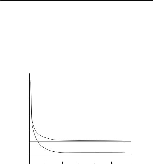
gent countries may significantly reduce the risk of portfolio returns. According to figure 16.5, drawn by Solnik (1999), that is indeed the case.
Figure 16.5 shows the total risk of domestically and internationally diversified portfolios as a function of the number of securities held. In this figure, 100 percent of risk as measured by standard deviation represents the typical risk of a single US security. As an investor increases the
410 INTERNATIONAL PORTFOLIO INVESTMENT
number of securities in a portfolio, the portfolio’s risk declines rapidly at first, then slowly approaches the systematic risk of the market expressed in the broken line. However, the addition of more securities beyond 15 or 20 reduces risk very little. The remaining risk – the part not affected by holding more US stocks – is called market risk, which is also known as systematic risk. Is there a way to lower portfolio risk even further? Only if we can lower the market risk. One way to lower the market risk is to hold stocks not traded on US stock exchanges.
Figure 16.5 illustrates a number of striking facts. First, the risk of a well-diversified US portfolio is only 27 percent of the typical risk of a single security. This relationship indicates that 73 percent of the risk associated with investing in a single security is diversifiable in a fully diversified portfolio. Second, the addition of foreign stocks to a purely domestic portfolio reduces risk faster, as shown in the bottom curve. Third, a fully diversified international portfolio is less than half as risky as a fully diversified US portfolio. The addition of foreign stocks to a US portfolio reduces the US market risk even further, because foreign economies generally do not move one- for-one with the US economy. When the US economy is in a recession, foreign economies might be in expansion, and vice versa. This and other studies have established that security returns are less highly correlated internationally than domestically. This makes a strong case for international diversification as a means of risk diversification.
It is important to note that a fully diversified portfolio or an efficient portfolio is one that has zero, or very little, unsystematic risk. As illustrated in figure 16.5, an efficient international portfolio cuts the systematic risk of an efficient domestic portfolio in half. Domestic systematic risk declines because international diversification offsets US-specific reactions to worldwide events.
16.2.2Risk–return characteristics of capital markets
In the previous section, we discussed the benefits from diversifying international portfolios in terms of risk reduction, but we ignored return, another important aspect of investment. Certainly, investors simultaneously consider both risk and return in making investment decisions. In other words, they want to maximize expected return for a given amount of risk and minimize the amount of risk for a given level of return. Consequently, we ought to examine the risk–return characteristics of stock markets.
To ascertain the gains from international diversification, Morgan Stanley constructed portfolios that began with a 100 percent US portfolio and then they made it increasingly more international in increments of 10 percent. Switching from domestic to foreign investments was implemented by acquiring equally weighted portfolios of the 20 foreign indexes in Europe, Australia, and the Far East, using quarterly data for 71 years from 1926 to 1997. Figure 16.6 shows the performance of these portfolios in terms of risk–return trade-offs. As the proportion of the portfolio invested abroad increased, the return increased; in addition, the risk decreased until the proportion of foreign equities reached 50 percent of the portfolio. In other words, American investors could have enjoyed higher returns and less risk if they had held a portfolio that contained up to 50 percent invested in foreign stocks.
16.2.3The selection of an optimal portfolio
Before we discuss the selection of an optimal international portfolio, let us review the basic concept of bonds and stocks. Bonds are less risky than stocks. The standard deviation of bond
THE BENEFITS OF INTERNATIONAL DIVERSIFICATION
411
Annualized
return (%)
12.0
100% foreign
11.5
11.0
60% foreign, 40% US
10.5
10.0
30% foreign, 70% US
9.5
100% US
9.0
13
14
15
16
17
18
19
Annualized standard deviation of returns (%)
Figure 16.6 Risk–return trade-offs of international portfolios, 1926–97
Source: Morgan Stanley Capital Investment.
returns in any particular market is typically lower than the standard deviation of stock returns in that market. Certainly, lower risk implies lower mean rates of return for bonds compared with stocks. Table 16.4 shows risk–return statistics for bonds and stocks in various markets from the viewpoint of a US investor. In terms of the mean-variance decision rule, both bonds and stocks were efficient investments in each market. With the exception of Germany, all the bond means and standard deviations were lower than the corresponding stock statistics in each market.
Levy and Lerman (1988) compared the performance of various investment strategies for the 13 industrial countries listed in table 16.4. The right-hand curve of figure 16.7 is the efficient frontier when investors are restricted to stocks only. The left-hand curve is the efficient frontier when investors can buy both stocks and bonds. The middle curve is the efficient frontier when investors are restricted to bonds only. M(bs), M(b), and M(s) represent the optimal international portfolios for stocks and bonds, bonds, and stocks, respectively.
Levy and Lerman’s study found several advantages of international bond and stock diversification. A US investor who diversified across world bond markets could have earned almost twice as much as the mean rate of return on a US bond portfolio, having the same risk level. Moreover, the US stock market dominated the US bond market in terms of risk-adjusted returns. However, internationally diversified bond portfolios outperformed internationally diversified stock portfolios. Finally, internationally diversified portfolios of stocks and bonds outperformed internationally diversified portfolios of stocks only or bonds only.
Investment in US bonds is inefficient because, as shown in figure 16.7, its risk–return combination is deep inside the efficient frontier. The international bond portfolio M(b) in figure 16.7 outperformed US bonds in terms of mean rate of return at the same risk level. More specifically,


 W
W X
X Y
Y