

Литература / Advanced Digital Signal Processing and Noise Reduction (Saeed V. Vaseghi) / 09 - Power spectrum and correlation
.pdfAdvanced Digital Signal Processing and Noise Reduction, Second Edition.
Saeed V. Vaseghi
Copyright © 2000 John Wiley & Sons Ltd
ISBNs: 0-471-62692-9 (Hardback): 0-470-84162-1 (Electronic)
, P
|
jkω0t |
||
9 |
e |
||
kω t |
|||
0 |
|||
|
|||
|
|
5H |
|
|
|
|
|
POWER SPECTRUM AND CORRELATION
9.1Power Spectrum and Correlation
9.2Fourier Series: Representation of Periodic Signals
9.3Fourier Transform: Representation of Aperiodic Signals
9.4Non-Parametric Power Spectral Estimation
9.5Model-Based Power Spectral Estimation
9.6High Resolution Spectral Estimation Based on Subspace Eigen-Analysis
9.7Summary
The power spectrum reveals the existence, or the absence, of repetitive patterns and correlation structures in a signal process. These structural patterns are important in a wide range of applications such as data forecasting, signal coding, signal detection, radar, pattern
recognition, and decision-making systems. The most common method of spectral estimation is based on the fast Fourier transform (FFT). For many applications, FFT-based methods produce sufficiently good results. However, more advanced methods of spectral estimation can offer better frequency resolution, and less variance. This chapter begins with an introduction to the Fourier series and transform and the basic principles of spectral estimation. The classical methods for power spectrum estimation are based on periodograms. Various methods of averaging periodograms, and their effects on the variance of spectral estimates, are considered. We then study the maximum entropy and the model-based spectral estimation methods. We also consider several high-resolution spectral estimation methods, based on eigen-analysis, for the estimation of sinusoids observed in additive white noise.
264 |
Power Spectrum and Correlation |
9.1 Power Spectrum and Correlation
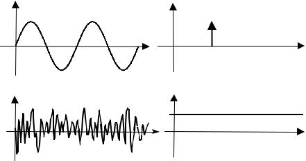
The power spectrum of a signal gives the distribution of the signal power among various frequencies. The power spectrum is the Fourier transform of the correlation function, and reveals information on the correlation structure of the signal. The strength of the Fourier transform in signal analysis and pattern recognition is its ability to reveal spectral structures that may be used to characterise a signal. This is illustrated in Figure 9.1 for the two extreme cases of a sine wave and a purely random signal. For a periodic signal, the power is concentrated in extremely narrow bands of frequencies, indicating the existence of structure and the predictable character of the signal. In the case of a pure sine wave as shown in Figure 9.1(a) the signal power is concentrated in one frequency. For a purely random signal as shown in Figure 9.1(b) the signal power is spread equally in the frequency domain, indicating the lack of structure in the signal.
In general, the more correlated or predictable a signal, the more concentrated its power spectrum, and conversely the more random or unpredictable a signal, the more spread its power spectrum. Therefore the power spectrum of a signal can be used to deduce the existence of repetitive structures or correlated patterns in the signal process. Such information is crucial in detection, decision making and estimation problems, and in systems analysis.
x(t) |
PXX(f) |
t |
f |
(a)
x(t) |
PXX(f) |
t |
f |
|
(b)
Figure 9.1 The concentration/spread of power in frequency indicates the correlated or random character of a signal: (a) a predictable signal, (b) a random signal.
Fourier Series: Representation of Periodic Signals |
265 |
 ,P
,P
sin(kω0t) cos(kω0t)
jk ω0t
e
Kω0t
5H
t
T0
(a) |
(b) |
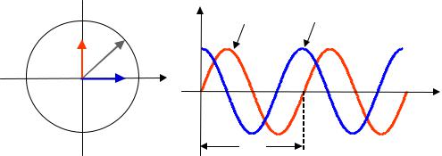
Figure 9.2 Fourier basis functions: (a) real and imaginary parts of a complex sinusoid, (b) vector representation of a complex exponential.
9.2 Fourier Series: Representation of Periodic Signals
The following three sinusoidal functions form the basis functions for the Fourier analysis:
x1(t) = cosω0t |
|
(9.1) |
x2 (t) = sinω0t |
|
(9.2) |
x3 (t) = cosω0t + j sinω0t = e |
jω0t |
(9.3) |
|
|
Figure 9.2(a) shows the cosine and the sine components of the complex exponential (cisoidal) signal of Equation (9.3), and Figure 9.2(b) shows a vector representation of the complex exponential in a complex plane with real (Re) and imaginary (Im) dimensions. The Fourier basis functions are periodic with an angular frequency of ω0 (rad/s) and a period of
T0=2π/ω0=1/F0, where F0 is the frequency (Hz). The following properties make the sinusoids the ideal choice as the elementary building block basis functions for signal analysis and synthesis:
(i) Orthogonality: two sinusoidal functions of different frequencies have the following orthogonal property:
266 |
|
|
Power Spectrum and Correlation |
|||
∞ |
1 |
∞ |
|
1 |
∞ |
|
∫sin(ω1t)sin(ω2t) dt = |
∫cos(ω1 |
+ ω2 ) dt + |
∫cos(ω1 − ω2 ) dt = 0 |
|||
2 |
|
|||||
−∞ |
−∞ |
2 |
−∞ |
|||
|
|
|
|
|
(9.4) |
|
For harmonically related sinusoids, the integration can be taken over one period. Similar equations can be derived for the product of cosines, or sine and cosine, of different frequencies. Orthogonality implies that the sinusoidal basis functions are independent and can be processed independently. For example, in a graphic equaliser, we can change the relative amplitudes of one set of frequencies, such as the bass, without affecting other frequencies, and in subband coding different frequency bands are coded independently and allocated different numbers of bits.
(ii)Sinusoidal functions are infinitely differentiable. This is important, as most signal analysis, synthesis and manipulation methods require the signals to be differentiable.
(iii)Sine and cosine signals of the same frequency have only a phase difference of π/2 or equivalently a relative time delay of a quarter of one period i.e. T0/4.
Associated with the complex exponential function e jω0t harmonically related complex exponentials of the form
[1,e± jω0t ,e± j2ω0t ,e± j3ω0t , ]
is a set of
(9.5)
The set of exponential signals in Equation (9.5) are periodic with a fundamental frequency ω0=2π/T0=2πF0, where T0 is the period and F0 is the
fundamental frequency. These signals form the set of basis functions for the Fourier analysis. Any linear combination of these signals of the form
∞ |
|
|
∑ ck e |
jkω0t |
(9.6) |
|
k =−∞
is also periodic with a period T0. Conversely any periodic signal x(t) can be synthesised from a linear combination of harmonically related exponentials. The Fourier series representation of a periodic signal is given by the following synthesis and analysis equations:
Fourier Transform: Representation of Aperiodic Signals |
267 |
|||
|
|
∞ |
|
|
x(t) = ∑ck e jkω0t k = −1,0,1, (synthesis equation) |
(9.7) |
|||
|
k=−∞ |
|
||
|
|
T / 2 |
|
|
ck = |
1 |
0∫ x(t)e− jkω0t dt k = −1,0,1, (analysis equation) |
(9.8) |
|
T |
||||
|
−T / 2 |
|
||
0 |
|
|||
|
|
0 |
|
|
The complex-valued coefficient ck conveys the amplitude (a measure of the strength) and the phase of the frequency content of the signal at kω0 (Hz). Note from Equation (9.8) that the coefficient ck may be interpreted as a measure of the correlation of the signal x(t) and the complex exponential
e− jkω0t .
9.3 Fourier Transform: Representation of Aperiodic Signals
The Fourier series representation of periodic signals consist of harmonically related spectral lines spaced at integer multiples of the fundamental frequency. The Fourier representation of aperiodic signals can be developed by regarding an aperiodic signal as a special case of a periodic signal with an infinite period. If the period of a signal is infinite then the signal does not repeat itself, and is aperiodic.
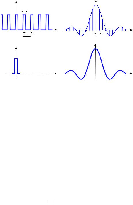
Now consider the discrete spectra of a periodic signal with a period of T0, as shown in Figure 9.3(a). As the period T0 is increased, the fundamental frequency F0=1/T0 decreases, and successive spectral lines become more closely spaced. In the limit as the period tends to infinity (i.e. as the signal becomes aperiodic), the discrete spectral lines merge and form a continuous spectrum. Therefore the Fourier equations for an aperiodic signal (known as the Fourier transform) must reflect the fact that the frequency spectrum of an aperiodic signal is continuous. Hence, to obtain the Fourier transform relation, the discrete-frequency variables and operations in the Fourier series Equations (9.7) and (9.8) should be replaced by their continuous-frequency counterparts. That is, the discrete summation sign Σ should be replaced by the continuous summation integral ∫, the discrete harmonics of the
fundamental frequency kF0 should be replaced by the continuous frequency variable f, and the discrete frequency spectrum ck should be replaced by a continuous frequency spectrum say X ( f ) .
268 |
Power Spectrum and Correlation |
|
x(t) |
|
|
c(k) |
|
|
|
|
|
|
Ton |
|
|
|
(a) |
Toff |
t |
1 |
k |
|
T0 |
|||
|
T0=Ton+Toff |
|
|
|
|
|
|
|
|
|
|
|
|
X(f) |
|
x(t) |
|
|
|
Toff = ∞
(b) |
t |
f |
|
||
|
|
Figure 9.3 (a) A periodic pulse train and its line spectrum. (b) A single pulse from the periodic train in (a) with an imagined “off” duration of infinity; its spectrum is the envelope of the spectrum of the periodic signal in (a).
The Fourier synthesis and analysis equations for aperiodic signals, the socalled Fourier transform pair, are given by
∞ |
|
|
x(t) = ∫ X ( f )e j2πft df |
(9.9) |
|
−∞ |
|
|
∞ |
− j2πft dt |
|
X ( f ) = ∫ x(t)e |
(9.10) |
|
−∞
Note from Equation (9.10), that X ( f ) may be interpreted as a measure of
the correlation of the signal x(t) and the complex sinusoid e− j2πft .
The condition for existence and computability of the Fourier transform integral of a signal x(t) is that the signal must have finite energy:
∞ |
|
∫ x(t) 2 dt < ∞ |
(9.11) |
−∞

Fourier Transform: Representation of Aperiodic Signals
x(0)  x(1)
x(1) 
x(2) 
.
.
.
x(N–2)  x(N – 1)
Discrete Fourier
Transform
N–1 |
–j |
2 πkn |
|
|
N |
||
X(k) = ∑ x(m) e |
|||
|
|||
m=0
269
 X(0)
X(0)
 X(1)
X(1)
 X(2)
X(2)
.
.
.
 X(N – 2)
  X(N– 1)
Figure 9.4 Illustration of the DFT as a parallel-input, parallel-output processor.
9.3.1 Discrete Fourier Transform (DFT)
For a finite-duration, discrete-time signal x(m) of length N samples, the discrete Fourier transform (DFT) is defined as N uniformly spaced spectral samples
N −1 |
− j(2π / N )mk , |
|
|
X (k) = ∑ x(m)e |
k = 0, . . ., N−1 |
(9.12) |
m=0
(see Figure9.4). The inverse discrete Fourier transform (IDFT) is given by
|
1 |
N −1 |
|
|
x(m) = |
∑ X (k)e j(2π / N )mk , m= 0, . . ., N−1 |
(9.13) |
||
|
||||
|
N k =0 |
|
||
From Equation (9.13), the direct calculation of the Fourier transform requires N(N−1) multiplications and a similar number of additions. Algorithms that reduce the computational complexity of the discrete Fourier transform are known as fast Fourier transforms (FFT) methods. FFT
methods utilise the periodic and symmetric properties of e− j2Œ to avoid redundant calculations.
9.3.2 Time/Frequency Resolutions, The Uncertainty Principle
Signals such as speech, music or image are composed of non-stationary (i.e. time-varying and/or space-varying) events. For example, speech is composed of a string of short-duration sounds called phonemes, and an

270 |
Power Spectrum and Correlation |
image is composed of various objects. When using the DFT, it is desirable to have high enough time and space resolution in order to obtain the spectral characteristics of each individual elementary event or object in the input signal. However, there is a fundamental trade-off between the length, i.e. the time or space resolution, of the input signal and the frequency resolution of the output spectrum. The DFT takes as the input a window of N uniformly spaced time-domain samples [x(0), x(1), …, x(N−1)] of duration ∆T=N.Ts,
and outputs N spectral samples [X(0), X(1), …, X(N−1)] spaced uniformly between zero Hz and the sampling frequency Fs=1/Ts Hz. Hence the
frequency resolution of the DFT spectrum ∆f, i.e. the space between successive frequency samples, is given by
û1 = |
1 |
= |
1 |
= |
Fs |
(9.14) |
|
NTs |
N |
||||
û% |
|
|
|
|||
Note that the frequency resolution ∆f and the time resolution ∆T are inversely proportional in that they cannot both be simultanously increased; in fact, ∆T∆f=1. This is known as the uncertainty principle.
9.3.3 Energy-Spectral Density and Power-Spectral Density
Energy, or power, spectrum analysis is concerned with the distribution of the signal energy or power in the frequency domain. For a deterministic discrete-time signal, the energy-spectral density is defined as
|
|
|
|
∞ |
|
2 |
|
|
|
|
|
||
X ( f ) |
|
2 |
= |
∑ x(m)e |
− j2πfm |
(9.15) |
|
||||||
|
|
|
|
m=−∞ |
|
|
The energy spectrum of x(m) may be expressed as the Fourier transform of the autocorrelation function of x(m):
X ( f ) |
|
2 = X ( f )X * ( f ) |
|
||
|
|
||||
|
|
∞ |
(m)e− j |
2πfm |
(9.16) |
= ∑r |
|
||||
|
|
xx |
|
|
|
m=−∞
where the variable rxx (m) is the autocorrelation function of x(m). The Fourier transform exists only for finite-energy signals. An important
Fourier Transform: Representation of Aperiodic Signals |
271 |
theoretical class of signals is that of stationary stochastic signals, which, as a consequence of the stationarity condition, are infinitely long and have infinite energy, and therefore do not possess a Fourier transform. For stochastic signals, the quantity of interest is the power-spectral density, defined as the Fourier transform of the autocorrelation function:
|
∞ |
(m)e− j2πfm |
|
P |
( f ) = ∑r |
(9.17) |
|
XX |
xx |
|
|
|
m=−∞ |
|
|
where the autocorrelation function rxx(m) is defined as |
|
||
rxx (m) = E [x(m)x(m + k)] |
(9.18) |
||
In practice, the autocorrelation function is estimated from a signal record of length N samples as
|
1 |
N −|m| |
−1 |
|
ˆ |
∑ x(k)x(k + m) , k =0, . . ., N–1 (9.19) |
|||
|
||||
rxx (m) = |
|
|||
|
N −| m | k =0 |
|
||
In Equation (9.19), as the correlation lag m approaches the record length N, the estimate of rˆxx (m) is obtained from the average of fewer samples and
has a higher variance. A triangular window may be used to “down-weight” the correlation estimates for larger values of lag m. The triangular window has the form
|
− |
| m | |
| m | ≤ N −1 |
|
1 |
|
, |
||
|
||||
w(m)= |
|
N |
(9.20) |
|
|
|
|
|
otherwise |
0, |
|
|
||
Multiplication of Equation (9.19) by the window of Equation (9.20) yields
ˆ |
1 |
N −|m| |
−1 |
|
∑ x(k)x(k + m) |
||
rxx (m)= |
N |
||
|
k =0 |
|
|
|
|
|
|
The expectation of the windowed correlation estimate rˆxx (m)
(9.21)
is given by

272 Power Spectrum and Correlation
|
[ˆ |
|
|
|
|
] |
|
1 |
|
N −|m|−1 |
[ |
|
] |
|
|
|
||||||
|
|
(m) |
= |
|
N |
|
|
|
∑ E |
|
|
|
|
|||||||||
|
E rxx |
|
|
|
|
|
x(k) x(k + m) |
|
|
|
|
|||||||||||
|
|
|
|
|
|
|
|
|
|
|
|
|
k=0 |
|
|
|
|
|
(9.22) |
|||
|
|
|
|
|
|
|
|
|
|
|
|
m |
|
|
|
|
|
|
|
|||
|
|
|
|
|
|
|
|
|
|
|
|
|
|
|
|
|
||||||
|
|
|
|
|
|
= |
1 |
− |
|
|
|
|
r |
|
(m) |
|
|
|
|
|||
|
|
|
|
|
|
|
|
|
|
|
|
|
|
|
||||||||
|
|
|
|
|
|
|
|
|
|
|
|
|
|
|
||||||||
|
|
|
|
|
|
|
|
|
|
|
|
N |
xx |
|
|
|
|
|
||||
|
|
|
|
|
|
|
|
|
|
|
|
|
|
|
|
|
|
|
||||
|
|
|
|
|
|
|
|
|
|
|
|
|
|
|
|
|
|
|
ˆ |
(m) is given by |
||
In Jenkins and Watts, it is shown that the variance of rxx |
||||||||||||||||||||||
[ˆ |
] |
≈ |
1 |
|
|
∞ |
[ |
2 |
|
|
|
|
|
|
|
|
|
] |
(9.23) |
|||
|
|
|
|
|
|
|
|
|
|
|
|
|
|
|
|
|||||||
Var rxx (m) |
|
|
|
∑ rxx (k) + rxx (k − m)rxx (k + m) |
|
|||||||||||||||||
|
|
|
|
N k=−∞ |
|
|
|
|
|
|
|
|
|
|
|
|
|
|||||
From Equations (9.22) and (9.23), rˆxx (m) is an asymptotically unbiased and consistent estimate.
9.4 Non-Parametric Power Spectrum Estimation
The classic method for estimation of the power spectral density of an N- sample record is the periodogram introduced by Sir Arthur Schuster in 1899. The periodogram is defined as
ˆ |
1 |
|
|
N −1 |
− j2πfm |
|
2 |
|
|
|
|||||
|
|
|
|
||||
PXX ( f ) = |
|
|
|
∑ x(m)e |
|
|
|
N |
|
|
|
||||
|
|
m=0 |
|
|
(9.24) |
||
|
|
|
|||||
= 1 X ( f ) 2
N
The power-spectral density function, or power spectrum for short, defined in Equation (9.24), is the basis of non-parametric methods of spectral estimation. Owing to the finite length and the random nature of most signals, the spectra obtained from different records of a signal vary randomly about an average spectrum. A number of methods have been developed to reduce the variance of the periodogram.
9.4.1 The Mean and Variance of Periodograms
The mean of the periodogram is obtained by taking the expectation of Equation (9.24):