Литература / Advanced Digital Signal Processing and Noise Reduction (Saeed V. Vaseghi) / 05 - Hidden Markov models

Advanced Digital Signal Processing and Noise Reduction, Second Edition.

Saeed V. Vaseghi

Copyright © 2000 John Wiley & Sons Ltd

ISBNs: 0-471-62692-9 (Hardback): 0-470-84162-1 (Electronic)

5

H E LL O

HIDDEN MARKOV MODELS

5.1Statistical Models for Non-Stationary Processes

5.2Hidden Markov Models

5.3Training Hidden Markov Models

5.4Decoding of Signals Using Hidden Markov Models

5.5HMM-Based Estimation of Signals in Noise

5.6Signal and Noise Model Combination and Decomposition

5.7HMM-Based Wiener Filters

5.8Summary

Hidden Markov models (HMMs) are used for the statistical modelling of non-stationary signal processes such as speech signals, image sequences and time-varying noise. An HMM models the time variations (and/or the space variations) of the statistics of a random process with a Markovian chain of state-dependent stationary subprocesses. An HMM is essentially a Bayesian finite state process, with a Markovian prior for modelling the transitions between the states, and a set of state probability density functions for modelling the random variations of the signal process within each state. This chapter begins with a brief introduction to continuous and finite state non-stationary models, before concentrating on the theory and applications of hidden Markov models. We study the various HMM structures, the Baum–Welch method for the maximum-likelihood training of the parameters of an HMM, and the use of HMMs and the Viterbi decoding algorithm for the classification and decoding of an unlabelled observation signal sequence. Finally, applications of the HMMs

for the enhancement of noisy signals are considered.

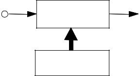
Figure 5.1 Illustration of a two-layered model of a non-stationary process.

5.1 Statistical Models for Non-Stationary Processes

A non-stationary process can be defined as one whose statistical parameters vary over time. Most “naturally generated” signals, such as audio signals, image signals, biomedical signals and seismic signals, are non-stationary, in that the parameters of the systems that generate the signals, and the environments in which the signals propagate, change with time.

A non-stationary process can be modelled as a double-layered stochastic process, with a hidden process that controls the time variations of the statistics of an observable process, as illustrated in Figure 5.1. In general, non-stationary processes can be classified into one of two broad categories:

(a)Continuously variable state processes.

(b)Finite state processes.

A continuously variable state process is defined as one whose underlying statistics vary continuously with time. Examples of this class of random processes are audio signals such as speech and music, whose power and spectral composition vary continuously with time. A finite state process is one whose statistical characteristics can switch between a finite number of stationary or non-stationary states. For example, impulsive noise is a binarystate process. Continuously variable processes can be approximated by an appropriate finite state process.

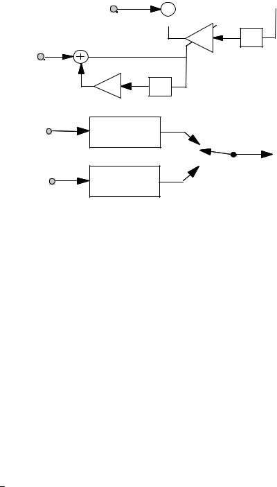
Figure 5.2(a) illustrates a non-stationary first-order autoregressive (AR) process. This process is modelled as the combination of a hidden stationary AR model of the signal parameters, and an observable time-varying AR model of the signal. The hidden model controls the time variations of the

Figure 5.3 (a) Illustration of a two-layered random process. (b) An HMM model of the process in (a).

5.2 Hidden Markov Models

A hidden Markov model (HMM) is a double-layered finite state process, with a hidden Markovian process that controls the selection of the states of an observable process. As a simple illustration of a binary-state Markovian process, consider Figure 5.3, which shows two containers of different mixtures of black and white balls. The probability of the black and the white balls in each container, denoted as PB and PW respectively, are as shown above Figure 5.3. Assume that at successive time intervals a hidden selection process selects one of the two containers to release a ball. The balls released are replaced so that the mixture density of the black and the white balls in each container remains unaffected. Each container can be considered as an underlying state of the output process. Now for an example assume that the hidden container-selection process is governed by the following rule: at any time, if the output from the currently selected

container is a white ball then the same container is selected to output the next ball, otherwise the other container is selected. This is an example of a Markovian process because the next state of the process depends on the current state as shown in the binary state model of Figure 5.3(b). Note that in this example the observable outcome does not unambiguously indicate the underlying hidden state, because both states are capable of releasing black and white balls.

In general, a hidden Markov model has N sates, with each state trained to model a distinct segment of a signal process. A hidden Markov model can be used to model a time-varying random process as a probabilistic Markovian chain of N stationary, or quasi-stationary, elementary subprocesses. A general form of a three-state HMM is shown in Figure 5.4. This structure is known as an ergodic HMM. In the context of an HMM, the term “ergodic” implies that there are no structural constraints for connecting any state to any other state.

A more constrained form of an HMM is the left–right model of Figure 5.5, so-called because the allowed state transitions are those from a left state to a right state and the self-loop transitions. The left–right constraint is useful for the characterisation of temporal or sequential structures of stochastic signals such as speech and musical signals, because time may be visualised as having a direction from left to right.

a11

Figure 5.4 A three-state ergodic HMM structure.

Figure 5.5 A 5-state left–right HMM speech model.

5.2.1 A Physical Interpretation of Hidden Markov Models

For a physical interpretation of the use of HMMs in modelling a signal process, consider the illustration of Figure 5.5 which shows a left–right HMM of a spoken letter “C”, phonetically transcribed as ‘s-iy’, together with a plot of the speech signal waveform for “C”. In general, there are two main types of variation in speech and other stochastic signals: variations in the spectral composition, and variations in the time-scale or the articulation rate. In a hidden Markov model, these variations are modelled by the state observation and the state transition probabilities. A useful way of interpreting and using HMMs is to consider each state of an HMM as a model of a segment of a stochastic process. For example, in Figure 5.5, state S1 models the first segment of the spoken letter “C”, state S2 models the second segment, and so on. Each state must have a mechanism to accommodate the random variations in different realisations of the segments that it models. The state transition probabilities provide a mechanism for

connection of various states, and for the modelling the variations in the duration and time-scales of the signals in each state. For example if a segment of a speech utterance is elongated, owing, say, to slow articulation, then this can be accommodated by more self-loop transitions into the state that models the segment. Conversely, if a segment of a word is omitted, owing, say, to fast speaking, then the skip-next-state connection accommodates that situation. The state observation pdfs model the probability distributions of the spectral composition of the signal segments associated with each state.

5.2.2 Hidden Markov Model as a Bayesian Model

A hidden Markov model M is a Bayesian structure with a Markovian state transition probability and a state observation likelihood that can be either a discrete pmf or a continuous pdf. The posterior pmf of a state sequence s of a model M, given an observation sequence X, can be expressed using Bayes’ rule as the product of a state prior pmf and an observation likelihood function:

where the observation sequence X is modelled by a probability density function PS|X,M(s|X,M).

The posterior probability that an observation signal sequence X was generated by the model M is summed over all likely state sequences, and

may also be weighted by the model prior PM (M ) :

The Markovian state transition prior can be used to model the time variations and the sequential dependence of most non-stationary processes. However, for many applications, such as speech recognition, the state observation likelihood has far more influence on the posterior probability than the state transition prior.

5.2.3 Parameters of a Hidden Markov Model

A hidden Markov model has the following parameters:

Number of states N. This is usually set to the total number of distinct, or elementary, stochastic events in a signal process. For example, in modelling a binary-state process such as impulsive noise, N is set to 2, and in isolated-word speech modelling N is set between 5 to 10.

State transition-probability matrix A={aij, i,j=1, ... N}. This provides a Markovian connection network between the states, and models the variations in the duration of the signals associated with each state. For a left–right HMM (see Figure 5.5), aij=0 for i>j, and hence the transition matrix A is upper-triangular.

State observation vectors {µi1, µi2, ..., µiM, i=1, ..., N}. For each state a set of M prototype vectors model the centroids of the signal space associated with each state.

State observation vector probability model. This can be either a discrete model composed of the M prototype vectors and their associated probability mass function (pmf) P={Pij(·); i=1, ..., N, j=1, ... M}, or it may be a continuous (usually Gaussian) pdf model F={fij(·); i=1, ...,

N, j=1, ..., M}.

Initial state probability vector π=[π1, π2, ..., πN].

5.2.4 State Observation Models

Depending on whether a signal process is discrete-valued or continuousvalued, the state observation model for the process can be either a discretevalued probability mass function (pmf), or a continuous-valued probability density function (pdf). The discrete models can also be used for the modelling of the space of a continuous-valued process quantised into a number of discrete points. First, consider a discrete state observation density model. Assume that associated with the ith state of an HMM there are M discrete centroid vectors [µi1, ..., µiM] with a pmf [Pi1, ..., PiM]. These centroid vectors and their probabilities are normally obtained through clustering of a set of training signals associated with each state.

Figure 5.6 Modelling a random signal space using (a) a discrete-valued pmf and (b) a continuous-valued mixture Gaussian density.

For the modelling of a continuous-valued process, the signal space associated with each state is partitioned into a number of clusters as in Figure 5.6. If the signals within each cluster are modelled by a uniform distribution then each cluster is described by the centroid vector and the cluster probability, and the state observation model consists of M cluster centroids and the associated pmf {µik, Pik; i=1, ..., N, k=1, ..., M}. In effect, this results in a discrete state observation HMM for a continuous-valued process. Figure 5.6(a) shows a partitioning, and quantisation, of a signal space into a number of centroids.

Now if each cluster of the state observation space is modelled by a continuous pdf, such as a Gaussian pdf, then a continuous density HMM results. The most widely used state observation pdf for an HMM is the mixture Gaussian density defined as

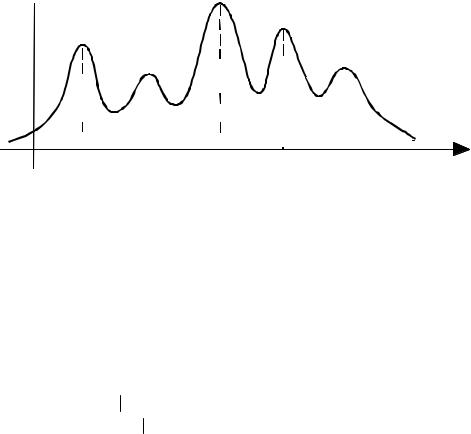
covariance matrix Σik, and Pik is a mixture weighting factor for the kth Gaussian pdf of the state i. Note that Pik is the prior probability of the kth mode of the mixture pdf for the state i. Figure 5.6(b) shows the space of a mixture Gaussian model of an observation signal space. A 5-mode mixture Gaussian pdf is shown in Figure 5.7.

f (x)

Figure 5.7 A mixture Gaussian probability density function.

5.2.5 State Transition Probabilities

The first-order Markovian property of an HMM entails that the transition probability to any state s(t) at time t depends only on the state of the process at time t–1, s(t–1), and is independent of the previous states of the HMM. This can be expressed as

Prob(s(t) = j s(t − 1) = i, s(t − 2) = k, , s(t − N) = l)

= Prob(s(t) = j s(t − 1) = i) =aij (5.7)

where s(t) denotes the state of HMM at time t. The transition probabilities provide a probabilistic mechanism for connecting the states of an HMM, and for modelling the variations in the duration of the signals associated with each state. The probability of occupancy of a state i for d consecutive time units, Pi(d), can be expressed in terms of the state self-loop transition probabilities aii as

From Equation (5.8), using the geometric series conversion formula, the mean occupancy duration for each state of an HMM can be derived as