Литература / Advanced Digital Signal Processing and Noise Reduction (Saeed V. Vaseghi) / 03 - Probability models

Advanced Digital Signal Processing and Noise Reduction, Second Edition.

Saeed V. Vaseghi

Copyright © 2000 John Wiley & Sons Ltd

ISBNs: 0-471-62692-9 (Hardback): 0-470-84162-1 (Electronic)

3 The small probability of collision of the Earth and a comet can become very great in adding over a long sequence of centuries. It is easy to picture the effects of this impact on the Earth. The axis and the motion of rotation have changed, the seas abandoning their old position...

Pierre-Simon Laplace

PROBABILITY MODELS

3.1Random Signals and Stochastic Processes

3.2Probabilistic Models

3.3Stationary and Non-stationary Processes

3.4Expected Values of a Process

3.5Some Useful Classes of Random Processes

3.6Transformation of a Random Process

3.7Summary

Probability models form the foundation of information theory. Information itself is quantified in terms of the logarithm of probability. Probability models are used to characterise and predict the occurrence of random events in such diverse areas of applications as

predicting the number of telephone calls on a trunk line in a specified period of the day, road traffic modelling, weather forecasting, financial data modelling, predicting the effect of drugs given data from medical trials, etc. In signal processing, probability models are used to describe the variations of random signals in applications such as pattern recognition, signal coding and signal estimation. This chapter begins with a study of the basic concepts of random signals and stochastic processes and the models that are used for the characterisation of random processes. Stochastic processes are classes of signals whose fluctuations in time are partially or completely random, such as speech, music, image, time-varying channels, noise and video. Stochastic signals are completely described in terms of a probability model, but can also be characterised with relatively simple statistics, such as the mean, the correlation and the power spectrum. We study the concept of ergodic stationary processes in which time averages obtained from a single realisation of a process can be used instead of ensemble averages. We consider some useful and widely used classes of random signals, and study the effect of filtering or transformation of a signal on its probability distribution.

3.1 Random Signals and Stochastic Processes

Signals, in terms of one of their most fundamental characteristics, can be classified into two broad categories: deterministic signals and random signals. Random functions of time are often referred to as stochastic signals. In each class, a signal may be continuous or discrete in time, and may have continuous-valued or discrete-valued amplitudes.

A deterministic signal can be defined as one that traverses a predetermined trajectory in time and space. The exact fluctuations of a deterministic signal can be completely described in terms of a function of time, and the exact value of the signal at any time is predictable from the functional description and the past history of the signal. For example, a sine wave x(t) can be modelled, and accurately predicted either by a second-order linear predictive model or by the more familiar equation x(t)=A sin(2πft+φ).

Random signals have unpredictable fluctuations; hence it is not possible to formulate an equation that can predict the exact future value of a random signal from its past history. Most signals such as speech and noise are at least in part random. The concept of randomness is closely associated with the concepts of information and noise. Indeed, much of the work on the processing of random signals is concerned with the extraction of information from noisy observations. If a signal is to have a capacity to convey information, it must have a degree of randomness: a predictable signal conveys no information. Therefore the random part of a signal is either the information content of the signal, or noise, or a mixture of both information and noise. Although a random signal is not completely predictable, it often exhibits a set of well-defined statistical characteristic values such as the maximum, the minimum, the mean, the median, the variance and the power spectrum. A random process is described in terms of its statistics, and most completely in terms of a probability model from which all its statistics can be calculated.

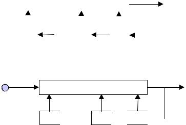
Example 3.1 Figure 3.1(a) shows a block diagram model of a deterministic discrete-time signal. The model generates an output signal x(m) from the P past samples as

where the function h1 may be a linear or a non-linear model. A functional description of the model h1 and the P initial sample values are all that is required to predict the future values of the signal x(m). For example for a sinusoidal signal generator (or oscillator) Equation (3.1) becomes

(a)

Random input e(m)

h2(·)

x(m)=h2(x(m–1), ..., x(m–P))

+e(m)

z –1 . . . z –1 z –1

(b)

Figure 3.1 Illustration of deterministic and stochastic signal models: (a) a deterministic signal model, (b) a stochastic signal model.

where the choice of the parameter a=2cos(2πF0 /Fs) determines the oscillation frequency F0 of the sinusoid, at a sampling frequency of Fs. Figure 3.1(b) is a model for a stochastic random process given by

where the random input e(m) models the unpredictable part of the signal x(m) , and the function h2 models the part of the signal that is correlated with the past samples. For example, a narrowband, second-order autoregressive process can be modelled as

where the choice of the parameters a1 and a2 will determine the centre frequency and the bandwidth of the process.

3.1.1 Stochastic Processes

The term “stochastic process” is broadly used to describe a random process that generates sequential signals such as speech or noise. In signal processing terminology, a stochastic process is a probability model of a class of random signals, e.g. Gaussian process, Markov process, Poisson process, etc. The classic example of a stochastic process is the so-called Brownian motion of particles in a fluid. Particles in the space of a fluid move randomly due to bombardment by fluid molecules. The random motion of each particle is a single realisation of a stochastic process. The motion of all particles in the fluid forms the collection or the space of different realisations of the process.

In this chapter, we are mainly concerned with discrete-time random processes that may occur naturally or may be obtained by sampling a continuous-time band-limited random process. The term “discrete-time stochastic process” refers to a class of discrete-time random signals, X(m), characterised by a probabilistic model. Each realisation of a discrete stochastic process X(m) may be indexed in time and space as x(m,s), where m is the discrete time index, and s is an integer variable that designates a space index to each realisation of the process.

3.1.2 The Space or Ensemble of a Random Process

The collection of all realisations of a random process is known as the ensemble, or the space, of the process. For an illustration, consider a random noise process over a telecommunication network as shown in Figure 3.2. The noise on each telephone line fluctuates randomly with time, and may be denoted as n(m,s), where m is the discrete time index and s denotes the line index. The collection of noise on different lines form the ensemble (or the space) of the noise process denoted by N(m)={n(m,s)}, where n(m,s) denotes a realisation of the noise process N(m) on the line s. The “true” statistics of a random process are obtained from the averages taken over the ensemble of many different realisations of the process. However, in many practical cases, only one realisation of a process is available. In Section 3.4, we consider the so-called ergodic processes in which time-averaged statistics, from a single realisation of a process, may be used instead of the ensemble-averaged statistics.

Notation The following notation is used in this chapter: X(m) denotes a random process, the signal x(m,s) is a particular realisation of the process X(m), the random signal x(m) is any realisation of X(m), and the collection

discrete-valued random variable X takes on a value of xi, P(X= xi), is called the probability mass function (pmf). For two such random variables X and Y, the probability of an outcome in which X takes on a value of xi and Y takes on a value of yj, P(X=xi, Y=yj), is called the joint probability mass function. The joint pmf can be described in terms of the conditional and the marginal probability mass functions as

PX ,Y (xi , y j ) = PY|X ( y j | xi )PX (xi )

(3.6)

= PX |Y (xi | y j )PY ( y j )

where PY | X (yj | xi ) is the probability of the random variable Y taking on a value of yj conditioned on X having taken a value of xi, and the so-called marginal pmf of X is obtained as

M

PX (xi ) = ∑ PX ,Y (xi , y j )

j=1

(3.7)

M

= ∑ PX |Y (xi | y j )PY ( y j ) j=1

where M is the number of values, or outcomes, in the space of the discrete random variable Y. From Equations (3.6) and (3.7), we have Bayes’ rule for the conditional probability mass function, given by

i=1

3.2.2Probability Density Function (pdf)

Now consider a continuous-valued random variable. A continuous-valued variable can assume an infinite number of values, and hence, the probability that it takes on a given value vanishes to zero. For a continuous-valued

random variable X the cumulative distribution function (cdf) is defined as the probability that the outcome is less than x as:

where Prob(·) denotes probability. The probability that a random variable X takes on a value within a band of ∆ centred on x can be expressed as

Since FX (x) increases with x, the pdf of x, which is the rate of change of FX(x) with x, is a non-negative-valued function; i.e. f X (x) ≥ 0. The integral of the pdf of a random variable X in the range ± ∞ is unity:

−∞

The conditional and marginal probability functions and the Bayes rule, of Equations (3.6)–(3.8), also apply to probability density functions of continuous-valued variables.

Now, the probability models for random variables can also be applied to random processes. For a continuous-valued random process X(m), the simplest probabilistic model is the univariate pdf fX(m)(x), which is the probability density function that a sample from the random process X(m) takes on a value of x. A bivariate pdf fX(m)X(m+n)(x1, x2) describes the probability that the samples of the process at time instants m and m+n take on the values x1, and x2 respectively. In general, an M-variate pdf

random process taking specific values at specific time instants. For an M- variate pdf, we can write

and the sum of the pdfs of all possible realisations of a random process is unity, i.e.

∞∞

The probability of a realisation of a random process at a specified time instant may be conditioned on the value of the process at some other time instant, and expressed in the form of a conditional probability density function as

If the outcome of a random process at any time is independent of its outcomes at other time instants, then the random process is uncorrelated. For an uncorrelated process a multivariate pdf can be written in terms of the products of univariate pdfs as

Discrete-valued stochastic processes can only assume values from a finite set of allowable numbers [x1, x2, ..., xn]. An example is the output of a binary message coder that generates a sequence of 1s and 0s. Discrete-time, discrete-valued, stochastic processes are characterised by multivariate probability mass functions (pmf) denoted as

The probability that a discrete random process X(m) takes on a value of xm at time instant m can be conditioned on the process taking on a value xn at some other time instant n, and expressed in the form of a conditional pmf as

3.3 Stationary and Non-Stationary Random Processes

Although the amplitude of a signal x(m) fluctuates with time m, the characteristics of the process that generates the signal may be time-invariant (stationary) or time-varying (non-stationary). An example of a nonstationary process is speech, whose loudness and spectral composition changes continuously as the speaker generates various sounds. A process is stationary if the parameters of the probability model of the process are timeinvariant; otherwise it is non-stationary (Figure 3.4). The stationarity property implies that all the parameters, such as the mean, the variance, the power spectral composition and the higher-order moments of the process, are time-invariant. In practice, there are various degrees of stationarity: it may be that one set of the statistics of a process is stationary, whereas another set is time-varying. For example, a random process may have a time-invariant mean, but a time-varying power.

Figure 3.4 Examples of a quasistationary and a non-stationary speech segment.