

Литература / Advanced Digital Signal Processing and Noise Reduction (Saeed V. Vaseghi) / 07 - Adaptive filters
.pdfAdvanced Digital Signal Processing and Noise Reduction, Second Edition. Saeed V. Vaseghi Copyright © 2000 John Wiley & Sons Ltd
ISBNs: 0-471-62692-9 (Hardback): 0-470-84162-1 (Electronic)
7 |
y(m) e(m) |
|||||
|
|
|
µ |
|
|
|
|
|
|
|
α w(m) |
||
wk(m+1)
α |
z –1 |
ADAPTIVE FILTERS
7.1State-Space Kalman Filters
7.2Sample-Adaptive Filters
7.3Recursive Least Square (RLS) Adaptive Filters
7.4The Steepest-Descent Method
7.5The LMS Filter
7.6Summary
Adaptive filters are used for non-stationary signals and environments, or in applications where a sample-by-sample adaptation of a process or a low processing delay is required.
Applications of adaptive filters include multichannel noise reduction, radar/sonar signal processing, channel equalization for cellular mobile phones, echo cancellation, and low delay speech coding. This chapter begins with a study of the state-space Kalman filter. In Kalman theory a state equation models the dynamics of the signal generation process, and an observation equation models the channel distortion and additive noise. Then we consider recursive least square (RLS) error adaptive filters. The RLS filter is a sample-adaptive formulation of the Wiener filter, and for stationary signals should converge to the same solution as the Wiener filter. In least square error filtering, an alternative to using a Wiener-type closedform solution is an iterative gradient-based search for the optimal filter coefficients. The steepest-descent search is a gradient-based method for searching the least square error performance curve for the minimum error filter coefficients. We study the steepest-descent method, and then consider the computationally inexpensive LMS gradient search method.

206
7.1 State-Space Kalman Filters
Adaptive Filters
The Kalman filter is a recursive least square error method for estimation of a signal distorted in transmission through a channel and observed in noise. Kalman filters can be used with time-varying as well as time-invariant processes. Kalman filter theory is based on a state-space approach in which a state equation models the dynamics of the signal process and an observation equation models the noisy observation signal. For a signal x(m) and noisy observation y(m), the state equation model and the observation model are defined as
x(m) =Φ (m, m −1)x(m −1) + e(m) |
(7.1) |
y(m) = Η (m)x(m) + n(m) |
(7.2) |
where
x(m) is the P-dimensional signal, or the state parameter, vector at time m, Φ(m, m–1) is a P × P dimensional state transition matrix that relates the
states of the process at times m–1 and m,
e(m) is the P-dimensional uncorrelated input excitation vector of the state equation,
Σee(m) is the P × P covariance matrix of e(m),
y(m) is the M-dimensional noisy and distorted observation vector, H(m) is the M × P channel distortion matrix,
n(m) is the M-dimensional additive noise process, Σnn(m) is the M × M covariance matrix of n(m).
The Kalman filter can be derived as a recursive minimum mean square error predictor of a signal x(m), given an observation signal y(m). The filter derivation assumes that the state transition matrix Φ(m, m–1), the channel
ˆ ( |
) |
|
(7.3) |
|
v(m) = y(m) − y |
m m −1 |
|
|
|
distortion matrix H(m), the covariance matrix Σee(m) of the state equation |
||||
input and the covariance matrix Σnn(m) of the additive noise are given. |
|
|||
ˆ( |
) |
to denote a prediction of |
||
In this chapter, we use the notation y |
m m − i |
|
||
y(m) based on the observation samples up to the time m–i. Now assume that yˆ(m m −1) is the least square error prediction of y(m) based on the observations [y(0), ..., y(m–1)]. Define a so-called innovation, or prediction error signal as
State-Space Kalman Filters
207
 n (m)
n (m)
e(m) |
x(m) |
|
|
+ |
|
y (m) |
|
|
|
||||
|
+ |
H(m) |
|
|
|
|
|
|
|
|
 Φ (m,m-1)
 Z -1
Z -1
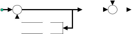
Figure 7.1 Illustration of signal and observation models in Kalman filter theory.
The innovation signal vector v(m) contains all that is unpredictable from the past observations, including both the noise and the unpredictable part of the signal. For an optimal linear least mean square error estimate, the innovation signal must be uncorrelated and orthogonal to the past observation vectors; hence we have
E [v(m) yT (m − k )]= 0 , |
k > 0 |
(7.4) |
and |
|
|
E[v(m)vT (k)]= 0 , |
m ≠ k |
(7.5) |
The concept of innovations is central to the derivation of the Kalman filter. The least square error criterion is satisfied if the estimation error is orthogonal to the past samples. In the following derivation of the Kalman filter, the orthogonality condition of Equation (7.4) is used as the starting point to derive an optimal linear filter whose innovations are orthogonal to the past observations.
Substituting the observation Equation (7.2) in Equation (7.3) and using
the relation |
[ |
|
|
|
ˆ( |
|
|
)] |
|
|
|
ˆ |
y(m) |
|
|
|
m |
|
|
||||
|
|
|
|
||||||||
y(m |
| m −1)=E |
|
x m |
|
−1 |
(7.6) |
|||||
|
|
ˆ( |
|
|
|
|
|
) |
|||
|
|
|
|
|
|
|
|||||
|
= H (m)x m |
m −1 |
|
|
|||||||
yields |
|
|
|
|
|
|
|
|
ˆ( |
|
) |
|
|
|
|
|
|
|
|
|
|
||
|
|
|
|
|
|
|
|
|
|
||
v(m) =H (m)x(m) + n(m) − H(m) x m |
|
m −1 |
|||||||||
|
~ |
|
|
|
|
|
|
|
|
|
(7.7) |
=H (m)x(m) + n(m) |
|
|
|
||||||||
where x˜(m) is the signal prediction error vector defined as |
|||||||||||
~ |
|
ˆ( |
|
) |
|
(7.8) |
|||||
|
|
|
|||||||||
x |
(m)=x(m) − x m |
|
m −1 |
|
|||||||
208 |
Adaptive Filters |
|
From Equation (7.7) the covariance matrix of the innovation signal is given |
||||||
by |
Σ vv (m) = E[v(m)vT (m)] |
|
|
|
||
|
|
|
|
|
(7.9) |
|
|
|
|
~~ |
T |
(m) + Σ nn (m) |
|
|
|
|
|
|
||
|
|
|
= H (m) Σ xx (m)H |
|
|
|
where Σ x˜x˜ |
(m) is the covariance matrix of the prediction error |
˜ |
||||
x(m) . Let |
||||||
xˆ(m +1 |
|
m) denote the least square error prediction of the signal x(m+1). |
||||
|
||||||
Now, the prediction of x(m+1), based on the samples available up to the time m, can be expressed recursively as a linear combination of the prediction based on the samples available up to the time m–1 and the innovation signal at time m as
ˆ( |
|
) |
ˆ( |
|
|
) |
+ K (m)v(m) |
(7.10) |
|||
|
|
||||||||||
x m + 1 |
|
m |
= x m +1 |
|
m −1 |
||||||
where the P × M matrix K(m) is the |
Kalman gain matrix. Now, from |
||||||||||
Equation (7.1), we have |
|
|
|
|
|
|
|
|
|||
ˆ( |
|
+1 |
|
) |
|
|
|
ˆ( |
|
) |
(7.11) |
|
|
|
|
|
|
||||||
x m |
|
m −1 |
=Φ (m +1, m)x m |
|
m −1 |
||||||
Substituting Equation (7.11) in (7.10) gives a recursive prediction equation as
ˆ( |
|
) |
ˆ( |
|
) |
+ K (m)v(m) |
(7.12) |
|
|
||||||
x m +1 |
|
m |
= Φ (m +1, m)x m |
|
m −1 |
To obtain a recursive relation for the computation and update of the Kalman gain matrix, we multiply both sides of Equation (7.12) by vT(m) and take the expectation of the results to yield
[ˆ ( |
m +1 |
|
) T |
] |
[ |
ˆ ( |
m |
|
m −1 |
) |
v |
T |
] |
[ |
T |
(m) |
] |
|
|
||||||||||||||||
E x |
|
m v |
(m) |
= E Φ (m +1, m) x |
|
|
|
(m) + K (m)E v(m)v |
|
|
|||||||
(7.13) Owing to the required orthogonality of the innovation sequence and the past samples, we have
[ˆ( |
|
) T |
] |
(7.14) |
|
||||
E x m |
|
m −1 v |
(m) =0 |
Hence, from Equations (7.13) and (7.14), the Kalman gain matrix is given by
[ˆ ( |
m + 1 |
|
) |
v |
T |
] −1 |
(m) |
(7.15) |
|
||||||||
K (m)=E x |
|
m |
|
(m) Σ vv |
State-Space Kalman Filters
209
The first term on the right-hand side of Equation (7.15) can be expressed as
[ˆ |
T |
] |
[ ( |
) |
~ |
|
|
|
|
|
|
|
T |
|
|
] |
|
|
|
|
|
|
|
||
E x(m +1 |
m)v |
|
(m) |
=E (x m +1 − x(m +1 |
m))v |
|
|
(m) |
|
|
|
|
|
|
|
|
|||||||||
|
|
|
=E[x(m + 1)vT (m)] |
|
|
|
|
|
|
|
|
|
|
|
|
|
|
|
|||||||
|
|
|
|
[( |
+1, m)x(m)+e(m |
+1) |
) |
|
|
ˆ |
|
|
m |
|
T ] |
||||||||||
|
|
|
|
|
|
|
|
|
|||||||||||||||||
|
|
|
= E Φ (m |
|
|
(y(m)− y(m |
−1)) |
||||||||||||||||||
|
|
|
|
[[ |
|
ˆ |
|
|
|
~ |
|
|
|
|
] |
|
|
~ |
(m |
|
T ] |
||||
|
|
|
|
|
|
|
|
|
|
|
|
|
|||||||||||||
|
|
|
= E Φ (m +1, m)(x(m |
|
m −1)+ x(m |
m −1)) (H (m)x |
|
m −1)+ n(m)) |
|||||||||||||||||
|
|
|
|
|
~ |
(m |
|
~ |
|
(m |
|
m −1)]H |
|
(m) |
|
|
|
|
|||||||
|
|
|
|
|
|
|
|
|
|
|
|
|
|||||||||||||
|
|
|
=Φ (m +1, m)E[x |
|
m −1)x |
T |
|
T |
|
|
|
|
|||||||||||||
|
|
|
|
|
|
|
|
|
|
|
|
|
|
|
|
|
|
|
|
|
|
|
|
||
In developing the successive lines of Equation (7.16), following relations:
E[e(m + 1)( y(m)− yˆ (m| m −1))T ]= 0
ˆ |
˜ |
( |
) |
|
m|m − 1 |
||
x(m) = x(m| m − 1)+ x |
|||
[ ˆ |
~( |
m| m −1 |
)] |
= 0 |
E x(m | m −1) x |
|
|||
(7.16) we have used the
(7.17)
(7.18)
(7.19)
(7.20)
and we have also used the assumption that the signal and the noise are uncorrelated. Substitution of Equations (7.9) and (7.16) in Equation (7.15) yields the following equation for the Kalman gain matrix:
( ) = |
+ |
~~ |
(m)H |
T |
[ |
~~ |
(m)H |
T |
(m) |
+ |
Σ nn (m) |
]−1 |
K m Φ (m |
|
1, m)Σ xx |
|
(m) H(m)Σ xx |
|
|
(7.21) |
|||||
where Σ (m) is the covariance matrix of x˜(m|m − 1) . To derive a recursive relation for Σ
~( |
) |
( ) |
ˆ( |
) |
x m |
m −1 |
= x m |
− x m |
m −1 |
the signal prediction error x˜x˜ (m), we consider
(7.22)
Substitution of Equation (7.1) and (7.12) in Equation (7.22) and rearrangement of the terms yields
~( |
m | m −1 |
) |
[ |
] |
|
ˆ ( |
m −1 |
|
m − 2 |
) |
+ K (m −1)v(m −1) |
] |
|
|
|||||||||||
x |
|
= Φ (m, m −1) x(m −1) |
+ e(m) |
− [Φ (m, m −1) x |
|
|
||||||
|
|
|
~ |
+ e(m) − K (m −1) H (m − |
~ |
|
|
+ K (m −1)n(m −1) |
|
|||
|
|
|
= Φ (m, m −1) x(m −1) |
1) x (m −1) |
|
|||||||
|
|
|
|
|
~ |
(m −1)+ e(m) + K (m |
−1)n(m −1) |
|
||||
|
|
|
= [Φ (m, m −1) − K (m −1) H (m −1)]x |
|
||||||||
|
|
|
|
|
|
|
|
|
|
|
(7.23) |
|
210 |
Adaptive Filters |
|
From Equation (7.23) we can derive the following recursive relation for the variance of the signal prediction error
Σ xx |
|
T |
T |
(m −1) |
(m)= L(m)Σ xx (m −1)L (m) + Σ ee (m) + K(m −1)Σ nn (m −1)K |
|
|||
~~ |
~~ |
|
|
|
where the P × P matrix L(m) is defined as |
|
(7.24) |
||
|
|
|||
|
L(m) = [Φ (m, m −1) − K (m −1)H (m −1)] |
|
(7.25) |
|
Kalman Filtering Algorithm
Input: observation vectors {y(m)}
Output: state or signal vectors { xˆ(m) }
Initial conditions:
Σ xx (0) = δI |
(7.26) |
~~ |
|
|
|
|
ˆ( |
|
|
) |
|
|
|
|
|
|
(7.27) |
|
|
|
|
|
|
|
|
|
|
|
|||
|
|
|
x 0 |
−1 = 0 |
|
|
|
|
|
||||
For m = 0, 1, ... |
|
|
|
|
|
|
|
|
|
|
|
||
Innovation signal: |
|
|
|
|
ˆ |
|
− 1) |
|
|
|
|||
|
|
|
|
|
|
|
|
|
|
(7.28) |
|||
|
|
v(m) = y(m ) − H(m)x(m|m |
|
|
|||||||||
Kalman gain: |
|
|
|
[ |
|
|
|
|
|
|
]−1 |
||
|
|
|
~~ |
T |
|
|
~~ |
(m)H |
T |
(m) + Σ nn (m) |
|||
K(m)=Φ (m +1,m)Σ xx (m)H |
|
|
(m) H(m)Σ xx |
|
|
||||||||
|
|
|
|
|
|
|
|
|
|
|
|
|
(7.29) |
Prediction update: |
|
|
|
ˆ( |
|
|
) |
+ K(m)v(m) |
|
||||
ˆ( |
m |
) |
|
|
|
|
|
(7.30) |
|||||
x |
+ 1|m |
= Φ (m + 1,m) x m|m − |
1 |
||||||||||
Prediction error correlation matrix update: |
|
|
|
|
|
||||||||
|
|
L(m+1) = [Φ (m + 1,m) − K(m)H(m)] |
(7.31) |
||||||||||
Σ xx (m +1)=L(m + |
1)Σ xx (m)L(m +1) |
T |
+ Σ ee (m +1) + K (m)Σ nn(m)K(m) |
||||||||||
~~ |
|
|
~~ |
|
|
|
|
|
|
|
|
|
|
|
|
|
|
|
|
|
|
|
|
|
|
|
(7.32) |
Example 7.1 Consider the Kalman filtering of a first-order AR process x(m) observed in an additive white Gaussian noise n(m). Assume that the signal generation and the observation equations are given as
x(m)= a(m)x(m − 1) + e(m) |
(7.33) |
State-Space Kalman Filters |
211 |
|
|
y(m)= x(m) + n(m) |
(7.34) |
Let σe2(m) and σn2(m) denote the variances of the excitation signal e(m)
and the noise n(m) respectively. Substituting Φ(m+1,m)=a(m) and H(m)=1 in the Kalman filter equations yields the following Kalman filter algorithm:
Initial conditions:
2 |
(0) |
= δ |
(7.35) |
σ ~ |
|||
x |
|
|
|
ˆ( |
|
) |
= 0 |
|
|
|
|
(7.36) |
|
|
|
|
|
||||
x 0 |
−1 |
|
|
|
|
|||
For m = 0, 1, ... |
|
|
|
|
|
|
|
|
Kalman gain: |
|
|
|
|
|
|
|
|
|
|
|
|
2 |
(m) |
|
|
|
|
|
a(m + 1)σ x |
|
|
||||
k(m)= |
|
|
~ |
|
|
|
(7.37) |
|
|
2 |
|
2 |
(m) |
|
|||
|
σ ~ (m) + σ |
n |
|
|
|
|||
|
|
x |
|
|
|
|
|
|
Innovation signal: |
|
|
ˆ( |
|
|
|
) |
|
|
|
|
|
|
|
(7.38) |
||
v(m)= y(m)− x m | m − 1 |
|
|||||||
Prediction signal update: |
|
|
|
|
|
|
|
|
ˆ |
|
|
ˆ |
|
|
|
|
(7.39) |
x(m + 1| m)= a(m + |
1)x(m|m − 1)+ k(m)v(m) |
|||||||
Prediction error update: |
|
|
|
|
|
|
|
|
σ ˜x2 (m + 1) = [a(m + 1) − k(m)]2 σx˜2(m) + σe2 (m + 1) + k2 (m)σn2(m) |
(7.40) |
|||||||
where σ 2x˜ (m) is the variance of the prediction error signal.
Example 7.2 Recursive estimation of a constant signal observed in noise.
Consider the estimation of a constant signal observed in a random noise. The state and observation equations for this problem are given by
x(m)= x(m − 1) = x |
(7.41) |
y(m)= x + n(m) |
(7.42) |
Note that Φ(m,m–1)=1, state excitation e(m)=0 and H(m)=1. Using the Kalman algorithm, we have the following recursive solutions:
Initial Conditions:
σ ˜x2(0) = δ |
(7.43) |
||
xˆ(0 |
|
−1) = 0 |
(7.44) |
|
|||
212
For m = 0, 1, ...
Kalman gain:
|
|
|
|
|
2 |
|
|
|
|
|
|
|
|
|
|
|
|
|
|
σ x (m) |
|
|
|
|
|
|
|
|
|
|
k(m)= |
|
|
~ |
|
|
|
|
|
|
|
|
|
|
|
|
2 |
(m) + σ |
2 |
(m) |
|
|
|
|
|||||
|
|
|
σ ~ |
n |
|
|
|
|
||||||
|
|
|
|
x |
|
|
|
|
|
|
|
|
||
Innovation signal: |
|
|
|
|
ˆ |
( |
|
|
) |
|
|
|
||
|
|
|
|
|
|
|
|
|
|
|||||
|
|
v(m) = y(m)−x m| m −1 |
|
|
|
|||||||||
Prediction signal update: |
|
|
|
|
|
|
|
|
|
|
|
|
|
|
|
ˆ |
|
|
|
ˆ |
|
|
|
|
|
|
|
|
|
|
x(m |
+ 1| m)=x(m | m −1)+ k(m)v(m) |
|
|||||||||||
Prediction error update: |
|
|
|
|
|
|
|
|
|
|
|
|
|
|
2 |
(m +1)=[1 |
|
2 |
|
2 |
(m)+ k |
2 |
(m)σ |
2 |
(m) |
||||
σ ~ |
− k(m)] σ |
~ |
|
n |
||||||||||
x |
|
|
|
|
|
|
x |
|
|
|
|
|
|
|
Adaptive Filters
(7.45)
(7.46)
(7.47)
(7.48)
7.2 Sample-Adaptive Filters
Sample adaptive filters, namely the RLS, the steepest descent and the LMS, are recursive formulations of the least square error Wiener filter. Sampleadaptive filters have a number of advantages over the block-adaptive filters of Chapter 6, including lower processing delay and better tracking of nonstationary signals. These are essential characteristics in applications such as echo cancellation, adaptive delay estimation, low-delay predictive coding, noise cancellation, radar, and channel equalisation in mobile telephony, where low delay and fast tracking of time-varying processes and environments are important objectives.
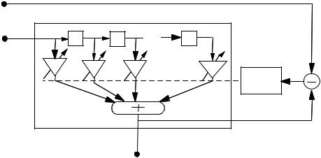
Figure 7.2 illustrates the configuration of a least square error adaptive filter. At each sampling time, an adaptation algorithm adjusts the filter coefficients to minimise the difference between the filter output and a desired, or target, signal. An adaptive filter starts at some initial state, and then the filter coefficients are periodically updated, usually on a sample-by- sample basis, to minimise the difference between the filter output and a desired or target signal. The adaptation formula has the general recursive form:
next parameter estimate = previous parameter estimate + update(error)
where the update term is a function of the error signal. In adaptive filtering a number of decisions has to be made concerning the filter model and the adaptation algorithm:
Recursive Least Square (RLS) Adaptive Filters
213
(a)Filter type: This can be a finite impulse response (FIR) filter, or an infinite impulse response (IIR) filter. In this chapter we only consider FIR filters, since they have good stability and convergence properties and for this reason are the type most often used in practice.
(b)Filter order: Often the correct number of filter taps is unknown. The filter order is either set using a priori knowledge of the input and the desired signals, or it may be obtained by monitoring the changes in the error signal as a function of the increasing filter order.
(c)Adaptation algorithm: The two most widely used adaptation algorithms are the recursive least square (RLS) error and the least mean square error (LMS) methods. The factors that influence the choice of the adaptation algorithm are the computational complexity, the speed of convergence to optimal operating condition, the minimum error at convergence, the numerical stability and the robustness of the algorithm to initial parameter states.
7.3 Recursive Least Square (RLS) Adaptive Filters
The recursive least square error (RLS) filter is a sample-adaptive, timeupdate, version of the Wiener filter studied in Chapter 6. For stationary signals, the RLS filter converges to the same optimal filter coefficients as the Wiener filter. For non-stationary signals, the RLS filter tracks the time variations of the process. The RLS filter has a relatively fast rate of convergence to the optimal filter coefficients. This is useful in applications such as speech enhancement, channel equalization, echo cancellation and radar where the filter should be able to track relatively fast changes in the signal process.
In the recursive least square algorithm, the adaptation starts with some initial filter state, and successive samples of the input signals are used to adapt the filter coefficients. Figure 7.2 illustrates the configuration of an adaptive filter where y(m), x(m) and w(m)=[w0(m), w1(m), ..., wP–1(m)] denote the filter input, the desired signal and the filter coefficient vector respectively. The filter output can be expressed as
ˆ |
= |
w |
T |
(m) y(m) |
(7.49) |
x(m) |
|
|
214 |
|
|
|
“Desired” or “target ” |
|
|
|
signal x(m) |
|
|
|
Input y(m) |
y(m–1) |
y(m–2) |
y(m-P-1) |
z–1 |
z –1 |
. . . |
z–1 |
w0 |
w1 |
w2 |
wP–1 |
Transversal |
filter |
|
|
|
|
^ |
|
|
|
x(m) |
|
Adaptive Filters
Adaptation e(m)
algorithm
Figure 7.2 Illustration of the configuration of an adaptive filter.
where xˆ(m) is an estimate of the desired signal x(m). The filter error signal is defined as
ˆ |
|
|
e(m) =x(m)−x(m) |
(7.50) |
|
=x(m)− wT |
||
(m) y(m) |
The adaptation process is based on the minimization of the mean square error criterion defined as
E[e2 (m)] = E |
[x(m) − wT (m) y(m)]2 |
|
|
=E[x2 (m)]−2wT (m)E [ y(m)x(m)]+ wT (m)E[ y(m) yT (m)] w(m)
=rxx (0) −2wT (m)ryx (m)+wT (m)Ryy (m)w(m)
(7.51) The Wiener filter is obtained by minimising the mean square error with respect to the filter coefficients. For stationary signals, the result of this minimisation is given in Chapter 6, Equation (6.10), as
w = R−yy1 ryx |
(7.52) |