

Литература / Advanced Digital Signal Processing and Noise Reduction (Saeed V. Vaseghi) / 08 - Linear prediction models
.pdfAdvanced Digital Signal Processing and Noise Reduction, Second Edition.
Saeed V. Vaseghi
Copyright © 2000 John Wiley & Sons Ltd
ISBNs: 0-471-62692-9 (Hardback): 0-470-84162-1 (Electronic)
|
u(m) |
e(m) |
|
x(m) |
8 |
|
|
|
|
|
G |
|
|
|
|
aP |
a2 |
a1 |
|
|
x(m–P) z– 1 . . . |
x(m – 2) z– 1 |
x(m – 1) z– 1 |
LINEAR PREDICTION MODELS
8.1Linear Prediction Coding
8.2Forward, Backward and Lattice Predictors
8.3Short-term and Long-Term Linear Predictors
8.4MAP Estimation of Predictor Coefficients
8.5Sub-Band Linear Prediction
8.6Signal Restoration Using Linear Prediction Models
8.7Summary
Linear prediction modelling is used in a diverse area of applications, such as data forecasting, speech coding, video coding, speech recognition, model-based spectral analysis, model-based interpolation, signal restoration, and impulse/step event detection. In the statistical literature, linear prediction models are often referred to as autoregressive (AR) processes. In this chapter, we introduce the theory of linear prediction modelling and consider efficient methods for the computation of predictor coefficients. We study the forward, backward and lattice predictors, and consider various methods for the formulation and calculation of predictor coefficients, including the least square error and maximum a posteriori methods. For the modelling of signals with a quasiperiodic structure, such as voiced speech, an extended linear predictor that simultaneously utilizes the short and long-term correlation structures is introduced. We study sub-band linear predictors that are particularly useful for sub-band processing of noisy signals. Finally, the application of linear prediction in enhancement of noisy speech is considered. Further applications of linear prediction models in this book are in Chapter 11 on the interpolation of a sequence of lost samples, and in Chapters 12 and 13
on the detection and removal of impulsive noise and transient noise pulses.

228 |
|
|
|
Linear Prediction Models |
|
x(t) |
|
|
PXX(f) |
||
t |
|
|
|
|
f |
|
|
|
|
||
|
|
|
|
||
(a) |
|
|
|
|
|
x(t) |
|
|
PXX(f) |
||
|
t |
|
|
|
f |
|
|
|
|
|
|
(b) |
|
|
|
|
|
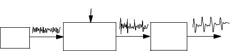
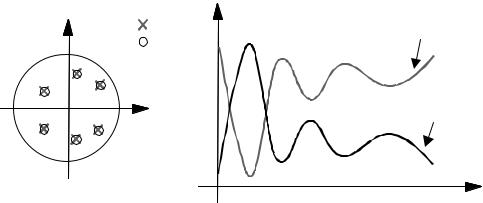
Figure 8.1 The concentration or spread of power in frequency indicates the predictable or random character of a signal: (a) a predictable signal;
(b)a random signal.
8.1Linear Prediction Coding
The success with which a signal can be predicted from its past samples depends on the autocorrelation function, or equivalently the bandwidth and the power spectrum, of the signal. As illustrated in Figure 8.1, in the time domain, a predictable signal has a smooth and correlated fluctuation, and in the frequency domain, the energy of a predictable signal is concentrated in narrow band/s of frequencies. In contrast, the energy of an unpredictable signal, such as a white noise, is spread over a wide band of frequencies.
For a signal to have a capacity to convey information it must have a degree of randomness. Most signals, such as speech, music and video signals, are partially predictable and partially random. These signals can be modelled as the output of a filter excited by an uncorrelated input. The random input models the unpredictable part of the signal, whereas the filter models the predictable structure of the signal. The aim of linear prediction is to model the mechanism that introduces the correlation in a signal.
Linear prediction models are extensively used in speech processing, in low bit-rate speech coders, speech enhancement and speech recognition. Speech is generated by inhaling air and then exhaling it through the glottis and the vocal tract. The noise-like air, from the lung, is modulated and shaped by the vibrations of the glottal cords and the resonance of the vocal tract. Figure 8.2 illustrates a source-filter model of speech. The source models the lung, and emits a random input excitation signal which is filtered by a pitch filter.
Linear Prediction Coding |
|
|
229 |
|
|
|
Pitch period |
|
|
Random |
|
Glottal (pitch) |
Vocal tract |
|
|
model |
model |
|
|
source |
Excitation |
P(z) |
H(z) |
Speech |
Figure 8.2 A source–filter model of speech production.
The pitch filter models the vibrations of the glottal cords, and generates a sequence of quasi-periodic excitation pulses for voiced sounds as shown in Figure 8.2. The pitch filter model is also termed the “long-term predictor” since it models the correlation of each sample with the samples a pitch period away. The main source of correlation and power in speech is the vocal tract. The vocal tract is modelled by a linear predictor model, which is also termed the “short-term predictor”, because it models the correlation of each sample with the few preceding samples. In this section, we study the short-term linear prediction model. In Section 8.3, the predictor model is extended to include long-term pitch period correlations.
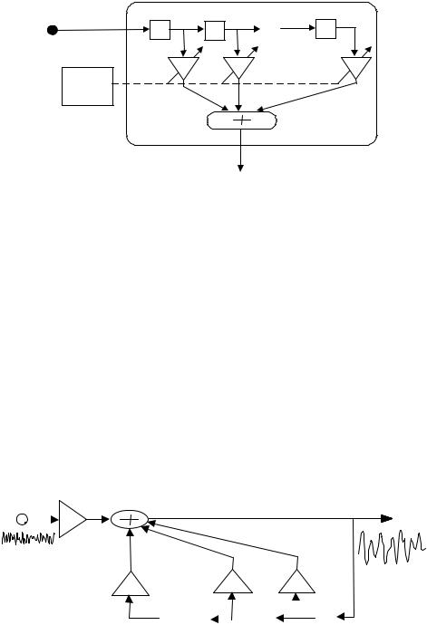
A linear predictor model forecasts the amplitude of a signal at time m, x(m), using a linearly weighted combination of P past samples [x(m−1), x(m−2), ..., x(m−P)] as
P |
|
ˆ |
(8.1) |
x(m) = ∑ak x(m − k) |
k =1
where the integer variable m is the discrete time index, xˆ(m) is the prediction of x(m), and ak are the predictor coefficients. A block-diagram implementation of the predictor of Equation (8.1) is illustrated in Figure 8.3.
The prediction error e(m), defined as the difference between the actual sample value x(m) and its predicted value xˆ(m) , is given by
ˆ |
|
e(m) = x(m) − x(m) |
|
P |
(8.2) |
= x(m) − ∑ akx(m − k) |
|
k=1
230 |
|
|
Linear Prediction Models |
Input x(m) |
x(m–1) |
x(m–2) |
x(m–P) |
z–1 |
z–1 |
. . . |
z–1 |
|
a1 |
a2 |
aP |
a = Rxx–1rxx |
|
|
|
Linear predictor
^
x(m)
Figure 8.3 Block-diagram illustration of a linear predictor.
For information-bearing signals, the prediction error e(m) may be regarded as the information, or the innovation, content of the sample x(m). From Equation (8.2) a signal generated, or modelled, by a linear predictor can be described by the following feedback equation
P |
|
x(m) = ∑ ak x(m − k) + e(m) |
(8.3) |
k =1
Figure 8.4 illustrates a linear predictor model of a signal x(m). In this model, the random input excitation (i.e. the prediction error) is e(m)=Gu(m), where u(m) is a zero-mean, unit-variance random signal, and G, a gain term, is the square root of the variance of e(m):
|
|
|
|
G=(E [e2 (m)])1/ 2 |
(8.4) |
u(m) |
|
e(m) |
x(m) |
||
|
|
|
|||
|
|
|
G |
|
|
|
|
|
|
|
|
aP |
|
a2 |
a1 |
||||||
|
|
|
|
|
|
|
|
|
|
|
z–1 |
. . . |
|
|
z–1 |
|
|
z–1 |
|
|
|
|
x(m–1) |
||||||
x(m–P) |
x(m–2) |
||||||||
|
|
|
|
||||||
|
|
|
|||||||
Figure 8.4 Illustration of a signal generated by a linear predictive model.
Linear Prediction Coding |
231 |
H(f)
pole-zero
f
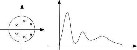
Figure 8.5 The pole–zero position and frequency response of a linear predictor.
where E[·] is an averaging, or expectation, operator. Taking the z-transform of Equation (8.3) shows that the linear prediction model is an all-pole digital filter with z-transfer function
H (z) = |
X (z) |
= |
|
G |
|
(8.5) |
|
|
P |
|
|||
|
U (z) |
|
|
|||
1 |
− ∑ak z |
−k |
||||
|
|
|
|
k =1 |
|
|
In general, a linear predictor of order P model up to P/2 resonance of the signal Spectral analysis using linear prediction
has P/2 complex pole pairs, and can spectrum as illustrated in Figure 8.5. models is discussed in Chapter 9.
8.1.1 Least Mean Square Error Predictor
The “best” predictor coefficients are normally obtained by minimising a mean square error criterion defined as
|
|
|
|
P |
|
2 |
|
|
|
2 |
|
|
|
|
|
|
|
E[e |
(m)]=E |
|
|
|
|
|
||
|
x(m)−∑ak x(m − k) |
|
|
|
||||
|
|
|
|
|
|
|
|
|
|
|
|
|
k=1 |
|
|
|
|
|
|
|
|
|
|
|
||
|
|
|
|
P |
|
|
P |
P |
|
|
=E[x2 (m)]−2∑ak E[x(m)x(m − k)]+ ∑ak ∑a j E[x(m − k)x(m − j)] |
||||||
|
|
|
|
k=1 |
|
|
k=1 |
j=1 |
=rxx (0) − 2rxxT a + aT Rxx a
(8.6)
232 |
Linear Prediction Models |
where Rxx =E[xxT] is the autocorrelation matrix of the input vector
xT=[x(m−1), x(m−2), . . ., x(m−P)], rxx=E[x(m)x] is the autocorrelation vector and aT=[a1, a2, . . ., aP] is the predictor coefficient vector. From
Equation (8.6), the gradient of the mean square prediction error with respect to the predictor coefficient vector a is given by
|
∂ |
|
|
|
|
|
|
|
|
||
|
|
|
E[e2 (m)] =− 2rxxT +2aT Rxx |
(8.7) |
|||||||
|
∂a |
||||||||||
where the gradient vector is defined as |
|
|
|
|
|||||||
|
|
|
∂ |
|
∂ |
|
∂ |
|
∂ |
T |
|
|
|
|
|
= |
|
, |
|
, , |
|
|
(8.8) |
|
|
∂ a |
∂ a1 |
∂ a2 |
|
||||||
|
|
|
|
|
∂ aP |
|
|||||
The least mean square error solution, obtained by setting Equation (8.7) to zero, is given by
Rxx a = rxx |
(8.9) |
From Equation (8.9) the predictor coefficient vector is given by |
|
a = Rxx−1 rxx |
(8.10) |
Equation (8.10) may also be written in an expanded form as |
|
a |
|
|
r |
(0) |
||
|
|
1 |
|
|
xx |
|
a2 |
|
|
rxx (1) |
|||
a |
3 |
|
= |
r |
(2) |
|
|
|
|
|
xx |
|
|
|
|
|
|
|
||
|
|
|
|
|
|
|
aP |
rxx (P − 1) |
|||||
rxx (1) rxx (0) rxx (1)
rxx (P − 2)
rxx (2)
rxx (1)
rxx (0)
rxx (P − 3)
|
r |
(P − |
1) |
−1 r |
(1) |
|
|||
|
xx |
|
|
|
|
xx |
|
|
|
rxx (P − |
2) |
rxx (2) |
|
||||||
|
r |
(P − |
3) |
|
r |
(3) |
|
(8.11) |
|
|
xx |
|
|
|
|
xx |
|
|
|
|
|
|
|
|
|
|
|
|
|
|
rxx (0) |
|
|
|
|
|
|
|
|
|
|
rxx (P) |
|
||||||
An alternative formulation of the least square error problem is as follows. For a signal block of N samples [x(0), ..., x(N−1)], we can write a set of N linear prediction error equations as
Linear Prediction Coding
|
e(0) |
|
|
x(0) |
|
x(−1) |
|
|
e(1) |
|
|
x(1) |
|
|
|
|
|
|
|
|
x(0) |
||
|
e(2) |
|
= |
x(2) |
|
− |
x(1) |
|
|
|
|
|
|
|
|
|
|
|
|
|
|
|
|
|
|
|
|
|
|
|
|
e(N − |
1) |
x(N − |
1) |
x(N − 2) |
|||
233
x(−2) |
x(−3) |
|
x(−P) |
a |
|
|
|
|
|
1 |
|
x(−1) |
x(−2) |
|
x(1 − P) |
a2 |
|
|
|
|
|
|
|
x(0) |
x(−1) |
|
x(2 − P) |
a3 |
|
|
|
|
|
|
|
x(N − 3) |
x(N − 4) |
x(N − P − |
|
|
|
1) aP |
|||||
(8.12) where xT= [x(−1), ..., x(−P)] is the initial vector. In a compact vector/matrix notation Equation (8.12) can be written as
e = x − Xa |
(8.13) |
Using Equation (8.13), the sum of squared prediction errors over a block of N samples can be expressed as
eTe= xT x− 2xT Xa− aT X T Xa |
(8.14) |
The least squared error predictor is obtained by setting the derivative of Equation (8.14) with respect to the parameter vector a to zero:
∂eTe |
= 0 |
(8.15) |
= − 2xT X − aT X T X |
||
∂a |
|
|
From Equation (8.15), the least square error predictor is given by |
|
|
a= (X T X )−1(X T x) |
|
(8.16) |
A comparison of Equations (8.11) and (8.16) shows that in Equation (8.16) the autocorrelation matrix and vector of Equation (8.11) are replaced by the time-averaged estimates as
|
1 |
N −1 |
|
|
rˆxx (m) = |
∑ x(k)x(k − m) |
(8.17) |
||
|
||||
|
N k=0 |
|
||
Equations (8.11) and ( 8.16) may be solved efficiently by utilising the regular Toeplitz structure of the correlation matrix Rxx. In a Toeplitz matrix,
234 |
Linear Prediction Models |
all the elements on a left–right diagonal are equal. The correlation matrix is also cross-diagonal symmetric. Note that altogether there are only P+1 unique elements [rxx(0), rxx(1), . . . , rxx(P)] in the correlation matrix and the cross-correlation vector. An efficient method for solution of Equation (8.10) is the Levinson–Durbin algorithm, introduced in Section 8.2.2.
8.1.2 The Inverse Filter: Spectral Whitening
The all-pole linear predictor model, in Figure 8.4, shapes the spectrum of the input signal by transforming an uncorrelated excitation signal u(m) to a correlated output signal x(m). In the frequency domain the input–output relation of the all-pole filter of Figure 8.6 is given by
X ( f ) = |
G U ( f ) |
= |
E( f ) |
(8.18) |
|
|
P |
|
|||
|
A( f ) |
|
|
||
|
|
|
1−∑ak e |
− j2πfk |
|
k=1
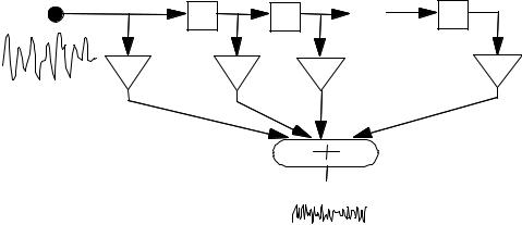
where X(f), E(f) and U(f) are the spectra of x(m), e(m) and u(m) respectively, G is the input gain factor, and A(f) is the frequency response of the inverse predictor. As the excitation signal e(m) is assumed to have a flat spectrum, it follows that the shape of the signal spectrum X(f) is due to the frequency response 1/A(f) of the all-pole predictor model. The inverse linear predictor,
Input x(m) |
x(m–1) |
x(m–2) . . . |
x(m–P) |
z–1 |
z–1 |
z–1 |
|
1 |
–a1 |
–a2 |
–a |
P |
 e(m)
e(m)
Figure 8.6 Illustration of the inverse (or whitening) filter.
Linear Prediction Coding |
235 |
as the name implies, transforms a correlated signal x(m) back to an uncorrelated flat-spectrum signal e(m). The inverse filter, also known as the prediction error filter, is an all-zero finite impulse response filter defined as
ˆ |
|
e(m) = x(m) − x(m) |
|
P |
|
= x(m) − ∑ak x(m − k) |
(8.19) |
k=1
=(ainv )T x
where the inverse filter (ainv)T =[1, −a1, . . ., −aP]=[1, −a], and xT=[x(m), ..., x(m−P)]. The z-transfer function of the inverse predictor model is given by
P |
|
A(z) = 1 − ∑ak z− k |
(8.20) |
k =1
A linear predictor model is an all-pole filter, where the poles model the resonance of the signal spectrum. The inverse of an all-pole filter is an allzero filter, with the zeros situated at the same positions in the pole–zero plot as the poles of the all-pole filter, as illustrated in Figure 8.7. Consequently, the zeros of the inverse filter introduce anti-resonances that cancel out the resonances of the poles of the predictor. The inverse filter has the effect of flattening the spectrum of the input signal, and is also known as a spectral whitening, or decorrelation, filter.
Pole
Zero
Magnitude response
Inverse filter A(f)
Predictor 1/A(f)
f
Figure 8.7 Illustration of the pole-zero diagram, and the frequency responses of an all-pole predictor and its all-zero inverse filter.
236
8.1.3 The Prediction Error Signal
Linear Prediction Models
The prediction error signal is in general composed of three components:
(a)the input signal, also called the excitation signal;
(b)the errors due to the modelling inaccuracies;
(c)the noise.
The mean square prediction error becomes zero only if the following three conditions are satisfied: (a) the signal is deterministic, (b) the signal is correctly modelled by a predictor of order P, and (c) the signal is noise-free. For example, a mixture of P/2 sine waves can be modelled by a predictor of order P, with zero prediction error. However, in practice, the prediction error is nonzero because information bearing signals are random, often only approximately modelled by a linear system, and usually observed in noise. The least mean square prediction error, obtained from substitution of Equation (8.9) in Equation (8.6), is
P |
|
E(P) =E[e2 (m)]= rxx (0) − ∑ak rxx (k) |
(8.21) |
k=1
where E(P) denotes the prediction error for a predictor of order P. The prediction error decreases, initially rapidly and then slowly, with increasing predictor order up to the correct model order. For the correct model order, the signal e(m) is an uncorrelated zero-mean random process with an autocorrelation function defined as
|
2 |
=G |
2 |
if m = k |
(8.22) |
E[e(m)e(m − k)]= σ e |
|
||||
0 |
|
|
|
if m ≠ k |
|
where σe2 is the variance of e(m).
8.2 Forward, Backward and Lattice Predictors
The forward predictor model of Equation (8.1) predicts a sample x(m) from a linear combination of P past samples x(m−1), x(m−2), . . .,x(m−P).