

Литература / Advanced Digital Signal Processing and Noise Reduction (Saeed V. Vaseghi) / 10 - Interpolation
.pdfAdvanced Digital Signal Processing and Noise Reduction, Second Edition.
Saeed V. Vaseghi
Copyright © 2000 John Wiley & Sons Ltd
ISBNs: 0-471-62692-9 (Hardback): 0-470-84162-1 (Electronic)
10 |
? ?…? |
|
INTERPOLATION
10.1Introduction
10.2Polynomial Interpolation
10.3Model-Based Interpolation
10.4Summary
Interpolation is the estimation of the unknown, or the lost, samples of a signal using a weighted average of a number of known samples at the neighbourhood points. Interpolators are used in various forms in most signal processing and decision making systems. Applications of interpolators include conversion of a discrete-time signal to a continuoustime signal, sampling rate conversion in multirate communication systems, low-bit-rate speech coding, up-sampling of a signal for improved graphical representation, and restoration of a sequence of samples irrevocably distorted by transmission errors, impulsive noise, dropouts, etc. This chapter begins with a study of the basic concept of ideal interpolation of a band-limited signal, a simple model for the effects of a number of missing samples, and the factors that affect the interpolation process. The classical approach to interpolation is to construct a polynomial that passes through the known samples. In Section 10.2, a general form of polynomial interpolation and its special forms, Lagrange, Newton, Hermite and cubic spline interpolators, are considered. Optimal interpolators utilise predictive and statistical models of the signal process. In Section 10.3, a number of model-based interpolation methods are considered. These methods include maximum a posteriori interpolation, and least square error interpolation based on an autoregressive model. Finally, we consider time–frequency interpolation, and interpolation through searching an adaptive signal
codebook for the best-matching signal.

298 |
Interpolation |
10.1 Introduction
The objective of interpolation is to obtain a high-fidelity reconstruction of the unknown or the missing samples of a signal. The emphasis in this chapter is on the interpolation of a sequence of lost samples. However, first in this section, the theory of ideal interpolation of a band-limited signal is introduced, and its applications in conversion of a discrete-time signal to a continuous-time signal and in conversion of the sampling rate of a digital signal are considered. Then a simple distortion model is used to gain insight on the effects of a sequence of lost samples and on the methods of recovery of the lost samples. The factors that affect interpolation error are also considered in this section.
10.1.1 Interpolation of a Sampled Signal
A common application of interpolation is the reconstruction of a continuous-time signal x(t) from a discrete-time signal x(m). The condition for the recovery of a continuous-time signal from its samples is given by the Nyquist sampling theorem. The Nyquist theorem states that a band-limited signal, with a highest frequency content of Fc (Hz), can be reconstructed from its samples if the sampling speed is greater than 2Fc samples per second. Consider a band-limited continuous-time signal x(t), sampled at a rate of Fs samples per second. The discrete-time signal x(m) may be expressed as the following product:
x(t) |
sinc(πfct) |
x(t) |
|
|
|
Time |
|
|
time |
time |
time |
|
Low pass filter |
|
XP(f) |
(Sinc interpolator) |
X( f ) |
|
||
|
|
|
Frequency |
|
|
–F /2 |
0 F /2 |
freq |
–Fs/2 0 Fs/2 freq –Fc/2 0 Fc/2 freq |
s |
s |
|
|
Figure 10.1 Reconstruction of a continuous-time signal from its samples. In frequency domain interpolation is equivalent to low-pass filtering.

Introduction |
|
299 |
Original signal |
Zero inserted signal |
Interpolated signal |
time |
time |
time |
|
Figure 10.2 Illustration of up-sampling by a factor of 3 using a two-stage process of zero-insertion and digital low-pass filtering.
∞ |
|
x(m)= x(t) p(t)= ∑ x(t)δ (t − mTs ) |
(10.1) |
m=−∞
where p(t)=Σδ(t–mTs) is the sampling function and Ts=1/Fs is the sampling interval. Taking the Fourier transform of Equation (10.1), it can be shown that the spectrum of the sampled signal is given by
∞ |
|
X s ( f ) = X ( f )*P( f )= ∑ X ( f + kfs ) |
(10.2) |
k =−∞
where X(f) and P(f) are the spectra of the signal x(t) and the sampling function p(t) respectively, and * denotes the convolution operation. Equation (10.2), illustrated in Figure 10.1, states that the spectrum of a sampled signal is composed of the original base-band spectrum X(f) and the repetitions or images of X(f) spaced uniformly at frequency intervals of Fs=1/Ts. When the sampling frequency is above the Nyquist rate, the baseband spectrum X(f) is not overlapped by its images X(f±kFs), and the original signal can be recovered by a low-pass filter as shown in Figure 10.1. Hence the ideal interpolator of a band-limited discrete-time signal is an ideal low-pass filter with a sinc impulse response. The recovery of a continuous-time signal through sinc interpolation can be expressed as
∞ |
|
x(t)= ∑ x(m)Ts fc sinc[πfc (t − mTs )] |
(10.3) |
m=−∞
In practice, the sampling rate Fs should 2.5Fc, in order to accommodate interpolating low-pass filter.
be sufficiently greater than 2Fc, say the transition bandwidth of the
300 |
Interpolation |
10.1.2 Digital Interpolation by a Factor of I
Applications of digital interpolators include sampling rate conversion in multirate communication systems and up-sampling for improved graphical representation. To change a sampling rate by a factor of V=I/D (where I and D are integers), the signal is first interpolated by a factor of I, and then the interpolated signal is decimated by a factor of D.
Consider a band-limited discrete-time signal x(m) with a base-band spectrum X(f) as shown in Figure 10.2. The sampling rate can be increased by a factor of I through interpolation of I–1 samples between every two samples of x(m). In the following it is shown that digital interpolation by a factor of I can be achieved through a two-stage process of (a) insertion of I– 1 zeros in between every two samples and (b) low-pass filtering of the zeroinserted signal by a filter with a cutoff frequency of Fs/2I, where Fs is the sampling rate. Consider the zero-inserted signal xz(m) obtained by inserting I–1 zeros between every two samples of x(m) and expressed as
|
m |
m = 0,± I ,± 2 I , |
|||
x |
|
|
, |
||
|
|
||||
x z (m) = |
|
|
I |
(10.4) |
|
|
|
0, |
|
otherwise |
|
|
|
|
|||
The spectrum of the zero-inserted signal is related to the spectrum of the original discrete-time signal by
∞ |
|
|
|
X z ( f ) = ∑ xz (m)e |
− j2πfm |
|
|
m=−∞ |
|
|
|
∞ |
|
|
|
= ∑ x(m)e |
− j2πfmI |
(10.5) |
|
m=−∞
= X (I. f )
Equation (10.5) states that the spectrum of the zero-inserted signal Xz(f) is a frequency-scaled version of the spectrum of the original signal X(f). Figure 10.2 shows that the base-band spectrum of the zero-inserted signal is composed of I repetitions of the based band spectrum of the original signal. The interpolation of the zero-inserted signal is therefore equivalent to filtering out the repetitions of X(f) in the base band of Xz(f), as illustrated in Figure 10.2. Note that to maintain the real-time duration of the signal the
Introduction |
301 |
sampling rate of the interpolated signal xz(m) needs to be increased by a factor of I.
10.1.3 Interpolation of a Sequence of Lost Samples
In this section, we introduce the problem of interpolation of a sequence of M missing samples of a signal given a number of samples on both side of the gap, as illustrated in Figure 10.3. Perfect interpolation is only possible if the missing samples are redundant, in the sense that they carry no more information than that conveyed by the known neighbouring samples. This will be the case if the signal is a perfectly predictable signal such as a sine wave, or in the case of a band-limited random signal if the sampling rate is greater than M times the Nyquist rate. However, in many practical cases, the signal is a realisation of a random process, and the sampling rate is only marginally above the Nyquist rate. In such cases, the lost samples cannot be perfectly recovered, and some interpolation error is inevitable.
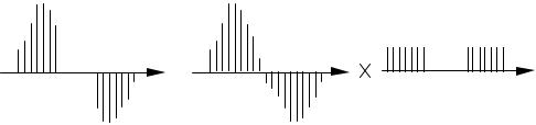
A simple distortion model for a signal y(m) with M missing samples, illustrated in Figure 10.3, is given by
y(m) = x(m)d(m)
= x(m) [1− r(m)] |
(10.6) |
|
|
where the distortion operator d(m) is defined as |
|
d(m)=1−r(m) |
(10.7) |
and r(m) is a rectangular pulse of duration M samples starting at the sampling time k:
y(m) x(m) d(m)
|
= |
m |
m |
m |
Figure 10.3 Illustration of a distortion model for a signal with a sequence of missing samples.

302
= 1, k ≤m≤k + M −1 r(m)
0, otherwise
In the frequency domain, Equation (10.6) becomes
Y ( f ) = X ( f ) * D( f )
=X ( f ) *[δ ( f )− R( f )]
=X ( f )− X ( f ) * R( f )
Interpolation
(10.8)
(10.9)
where D(f) is the spectrum of the distortion d(m), δ(f) is the Kronecker delta function, and R(f), the frequency spectrum of the rectangular pulse r(m), is given by
R( f ) = e |
− j2πf [k+(M −1) / 2] |
sin(πfM ) |
(10.10) |
|
|
sin(πf ) |
|
||
|
|
|
||
In general, the distortion d(m) is a non-invertible, many-to-one transformation, and perfect interpolation with zero error is not possible. However, as discussed in Section 10.3, the interpolation error can be minimised through optimal utilisation of the signal models and the information contained in the neighbouring samples.
Example 10.1 Interpolation of missing samples of a sinusoidal signal.
Consider a cosine waveform of amplitude A and frequency F0 with M missing samples, modelled as
y(m)= x(m) d(m) |
(10.11) |
|
= A(cos 2πf0m)[1− r(m)b] |
||
|
where r(m) is the rectangular pulse defined in Equation (10.7). In the frequency domain, the distorted signal can be expressed as
Y ( f ) = A [δ ( f − fo )+δ ( f + fo )]*[δ ( f )− R( f )] 2
= A [δ ( f − fo )+δ ( f + fo ) − R( f − fo ) −R( f + fo )]
(10.12)
2
where R(f) is the spectrum of the pulse r(m) as in Equation (10.9).
Introduction |
303 |
From Equation (10.12), it is evident that, for a cosine signal of frequency F0, the distortion in the frequency domain due to the missing samples is manifested in the appearance of sinc functions centred at ± F0. The distortion can be removed by filtering the signal with a very narrow band-pass filter. Note that for a cosine signal, perfect restoration is possible only because the signal has infinitely narrow bandwidth, or equivalently because the signal is completely predictable. In fact, for this example, the distortion can also be removed using a linear prediction model, which, for a cosine signal, can be regarded as a data-adaptive narrow band-pass filter.
10.1.4 The Factors That Affect Interpolation Accuracy
The interpolation accuracy is affected by a number of factors, the most important of which are as follows:
(a)The predictability, or correlation structure of the signal: as the correlation of successive samples increases, the predictability of a sample from the neighbouring samples increases. In general, interpolation improves with the increasing correlation structure, or equivalently the decreasing bandwidth, of a signal.
(b)The sampling rate: as the sampling rate increases, adjacent samples become more correlated, the redundant information increases, and interpolation improves.
(c)Non-stationary characteristics of the signal: for time-varying signals the available samples some distance in time away from the missing samples may not be relevant because the signal characteristics may have completely changed. This is particularly important in interpolation of a large sequence of samples.
(d)The length of the missing samples: in general, interpolation quality decreases with increasing length of the missing samples.
(e)Finally, interpolation depends on the optimal use of the data and the efficiency of the interpolator.
The classical approach to interpolation is to construct a polynomial interpolator function that passes through the known samples. We continue this chapter with a study of the general form of polynomial interpolation, and consider Lagrange, Newton, Hermite and cubic spline interpolators. Polynomial interpolators are not optimal or well suited to make efficient use of a relatively large number of known samples, or to interpolate a relatively large segment of missing samples.

304 |
Interpolation |
In Section 10.3, we study several statistical digital signal processing methods for interpolation of a sequence of missing samples. These include model-based methods, which are well suited for interpolation of small to medium sized gaps of missing samples. We also consider frequency–time interpolation methods, and interpolation through waveform substitution, which have the ability to replace relatively large gaps of missing samples.
10.2 Polynomial Interpolation
The classical approach to interpolation is to construct a polynomial interpolator that passes through the known samples. Polynomial interpolators may be formulated in various forms, such as power series, Lagrange interpolation and Newton interpolation. These various forms are mathematically equivalent and can be transformed from one into another. Suppose the data consists of N+1 samples {x(t0), x(t1), ..., x(tN)}, where x(tn) denotes the amplitude of the signal x(t) at time tn. The polynomial of order N that passes through the N+1 known samples is unique (Figure 10.4) and may be written in power series form as
ˆ |
= |
pN (t) |
= |
a0 |
+ |
a1t |
+ |
a2t |
2 + |
a3t |
3 + |
|
+ |
aN t |
N |
(10.13) |
x(t) |
|
|
|
|
|
|
|
|
where PN(t) is a polynomial of order N, and the ak are the polynomial coefficients. From Equation (10.13), and a set of N+1 known samples, a
x(t) |
|
|
|
|
|
|
|
|
P(ti)=x(t) |
t0 |
t1 |
t2 |
t3 |
t |
Figure 10.4 Illustration of an Interpolation curve through a number of samples.
Polynomial Interpolation |
305 |
system of N+1 linear equations with N+1 unknown coefficients can be formulated as
x(t |
0 |
) = |
a |
0 |
|
+ a t |
+ a |
2 |
t 2 + a |
3 |
t 3 |
+ + a |
N |
t N |
|
||||||||||
|
|
|
|
|
1 0 |
|
|
|
|
0 |
|
|
|
0 |
|
0 |
|
||||||||
x(t |
1 |
) = |
a |
0 |
|
+ a t |
+ a |
|
t |
2 |
+ a |
|
t 3 |
+ + a |
t N |
|
|||||||||
|
|
|
|
|
|
1 1 |
|
|
2 1 |
|
|
3 1 |
|
N |
1 |
(10.14) |
|||||||||
|
|
|
|
|
|
|
|
|
|
|
|
|
|
|
|
|
|
|
|
|
|
|
|||
|
|
|
|
|
|
|
|
|
|
|
|
|
|
|
|
|
|
|
|
|
|||||
x(t |
N |
) = |
a |
0 |
+ a t |
N |
+ a |
2 |
t 2 |
+ a |
3 |
t 3 + + a |
N |
t N |
|||||||||||
|
|
|
|
1 |
|
|
|
|
N |
|
|
|
|
N |
|
|
N |
||||||||
From Equation (10.14). the polynomial coefficients are given by
a |
0 |
|
|
|
t0 |
t |
2 |
t |
3 |
|
t |
N |
−1 x(t |
0 |
) |
|
|||
|
|
|
1 |
0 |
0 |
0 |
|
|
|
|
|
||||||||
|
a |
|
|
1 |
t |
t |
2 |
t |
3 |
|
t |
N |
|
x(t |
) |
|
|
||
|
1 |
|
|
|
|
|
1 |
|
|
||||||||||
|
|
|
|
|
|
1 |
1 |
1 |
|
1 |
|
|
|
|
|
(10.15) |
|||
a2 |
|
= 1 |
t2 |
t22 |
t23 |
t2N |
x(t |
2 ) |
|||||||||||
|
|
|
|
|
|
|
|
|
|
|
|
|
|
|
|||||
|
|
|
|
|
|
|
|
2 |
|
3 |
|
|
|
|
|
|
|
|
|
|
|
|
|
tN |
|
|
|
|
N |
|
|
|
|
||||||
aN |
1 |
tN |
tN |
tN |
x(tN ) |
|
|||||||||||||
The matrix in Equation (10.15) is called a Vandermonde matrix. For a large number of samples, N, the Vandermonde matrix becomes large and illconditioned. An ill-conditioned matrix is sensitive to small computational errors, such as quantisation errors, and can easily produce inaccurate results. There are alternative methods of implementation of the polynomial interpolator that are simpler to program and/or better structured, such as Lagrange and Newton methods. However, it must be noted that these variants of the polynomial interpolation also become ill-conditioned for a large number of samples, N.
10.2.1 Lagrange Polynomial Interpolation
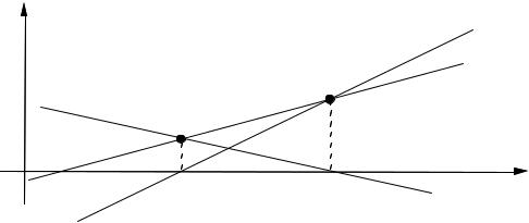
To introduce the Lagrange interpolation, consider a line interpolator passing through two points x(t0) and x(t1):
xˆ(t) = p |
(t) = x(t |
0 |
) + |
x(t1) − x(t0 ) |
(t −t |
0 |
) |
(10.16) |
|
||||||||
1 |
|
|
t1 − t0 |
|
||||
|
|
|
|
|
|
|
||
|
|
|
|
|
|
|
|
|
line slope
306 |
|
|
|
Interpolation |
x(t) |
|
|
t−t0 |
x(t ) |
|
|
|
|
|
|
1 |
|||
|
|
|
t1−t0 |
|
|
t−t1 |
x(t0 ) |
||
|
|
|||
|
t0 −t1 |
|||
t |
t |
t |
|
0 |
1 |
Figure 10.5 The Lagrange line interpolator passing through x(t0) and x(t1),
described in terms of the combination of two lines: one passing through (x(t0), t1) and the other through (x(t1), t0 ).
The line Equation (10.16) may be rearranged and expressed as
p (t) = |
t−t1 |
x(t |
0 |
) + |
t−t0 |
x(t ) |
(10.17) |
||
|
|
||||||||
1 |
t0 |
−t1 |
|
|
t1 |
−t0 |
1 |
|
|
|
|
|
|
|
|
||||
Equation (10.17) is in the form of a Lagrange polynomial. Note that the Lagrange form of a line interpolator is composed of the weighted combination of two lines, as illustrated in Figure 10.5.
In general, the Lagrange polynomial, of order N, passing through N+1 samples {x(t0), x(t1), ... x(tN)} is given by the polynomial equation
PN (t) = L0 (t)x(t0 ) + L1(t)x(t1) + + LN (t)x(tN ) |
(10.18) |
where each Lagrange coefficient LN(t) is itself a polynomial of degree N given by
|
(t −t0 ) (t −ti−1) (t −ti+1) (t −tN ) |
N |
t −tn |
|
|
Li (t) = |
|
= ∏ |
|
(10.19) |
|
(ti −t0 ) (ti −ti−1) (ti −ti+1) (ti −tN ) |
ti −tn |
||||
|
n=0 |
|
|||
|
|
n≠i |
|
|
Note that the ith Lagrange polynomial coefficient Li(t) becomes unity at the ith known sample point (i.e. Li(ti)=1), and zero at every other known sample