

Литература / Advanced Digital Signal Processing and Noise Reduction (Saeed V. Vaseghi) / 06 - Wiener filters
.pdfAdvanced Digital Signal Processing and Noise Reduction, Second Edition.
Saeed V. Vaseghi
Copyright © 2000 John Wiley & Sons Ltd
ISBNs: 0-471-62692-9 (Hardback): 0-470-84162-1 (Electronic)
6
WIENER FILTERS
6.1Wiener Filters: Least Square Error Estimation
6.2Block-Data Formulation of the Wiener Filter
6.3Interpretation of Wiener Filters as Projection in Vector Space
6.4Analysis of the Least Mean Square Error Signal
6.5Formulation of Wiener Filters in the Frequency Domain
6.6Some Applications of Wiener Filters
6.7The Choice of Wiener Filter Order
6.8Summary
Wiener theory, formulated by Norbert Wiener, forms the foundation of data-dependent linear least square error filters. Wiener filters play a central role in a wide range of applications
such as linear prediction, echo cancellation, signal restoration, channel equalisation and system identification. The coefficients of a Wiener filter are calculated to minimise the average squared distance between the filter output and a desired signal. In its basic form, the Wiener theory assumes that the signals are stationary processes. However, if the filter coefficients are periodically recalculated for every block of N signal samples then the filter adapts itself to the average characteristics of the signals within the blocks and becomes block-adaptive. A block-adaptive (or segment adaptive) filter can be used for signals such as speech and image that may be considered almost stationary over a relatively small block of samples. In this chapter, we study Wiener filter theory, and consider alternative methods of formulation of the Wiener filter problem. We consider the application of Wiener filters in channel equalisation, time-delay estimation and additive noise reduction. A case study of the frequency response of a Wiener filter, for additive noise reduction, provides useful insight into the operation of the filter. We also deal with some implementation issues of Wiener filters.
Least Square Error Estimation |
179 |
6.1 Wiener Filters: Least Square Error Estimation
Wiener formulated the continuous-time, least mean square error, estimation problem in his classic work on interpolation, extrapolation and smoothing of time series (Wiener 1949). The extension of the Wiener theory from continuous time to discrete time is simple, and of more practical use for implementation on digital signal processors. A Wiener filter can be an infinite-duration impulse response (IIR) filter or a finite-duration impulse response (FIR) filter. In general, the formulation of an IIR Wiener filter results in a set of non-linear equations, whereas the formulation of an FIR Wiener filter results in a set of linear equations and has a closed-form solution. In this chapter, we consider FIR Wiener filters, since they are relatively simple to compute, inherently stable and more practical. The main drawback of FIR filters compared with IIR filters is that they may need a large number of coefficients to approximate a desired response.
Figure 6.1 illustrates a Wiener filter represented by the coefficient vector w. The filter takes as the input a signal y(m), and produces an output signal xˆ(m) , where xˆ(m) is the least mean square error estimate of a desired or target signal x(m). The filter input–output relation is given by
P−1 |
|
ˆ |
|
x(m) = ∑ wk y(m − k ) |
(6.1) |
k =0 |
= w T y
where m is the discrete-time index, yT=[y(m), y(m–1), ..., y(m–P–1)] is the filter input signal, and the parameter vector wT=[w0, w1, ..., wP–1] is the
Wiener filter coefficient vector. In Equation (6.1), the filtering operation is expressed in two alternative and equivalent forms of a convolutional sum and an inner vector product. The Wiener filter error signal, e(m) is defined as the difference between the desired signal x(m) and the filter output signal xˆ(m) :
e(m) = x(m) − xˆ(m)
= x(m) − w T y (6.2)
In Equation (6.2), for a given input signal y(m) and a desired signal x(m), the filter error e(m) depends on the filter coefficient vector w.

180 |
|
|
Wiener Filters |
Input y(m) |
y(m–1) |
y(m–2) . . . |
z–1 y(m–P–1) |
z–1 |
z–1 |
||
w |
w |
w |
w |
0 |
1 |
2 |
P–1 |
w = R –1r |
|
|
|
yy xy |
|
|
|
FIR Wiener Filter
Desired signal x(m)
^
x(m)
Figure 6.1 Illustration of a Wiener filter structure.
To explore the relation between the filter coefficient vector w and the error signal e(m) we expand Equation (6.2) for N samples of the signals x(m) and y(m):
|
e(0) |
|
|
x(0) |
|
e(1) |
|
|
x(1) |
|
|
|
||
|
e(2) |
|
= |
x(2) |
|
|
|
|
|
|
|
|
|
|
|
|
|
|
|
e( N − |
1) |
x( N − |
||
|
|
|
y(0) |
|
|
|
y(1) |
|
|
|
|
|
− |
|
y(2) |
|
|
|
|
|
|
|
|
|
|
|
|
1)y( N − 1)
y(−1) y(−2)
y(0) y(−1)
y(1) |
y(0) |
y( N − 2) y( N − 3)
y( N
|
w |
|
|
0 |
|
|
w1 |
|
|
w2 |
|
|
|
|
|
|
|
|
|
|
− P) wP−1 |
|
|
(6.3)
In a compact vector notation this matrix equation may be written as
e= x −Yw |
(6.4) |
where e is the error vector, x is the desired signal vector, Y is the input signal matrix and Yw =xˆ is the Wiener filter output signal vector. It is assumed that the P initial input signal samples [y(–1), . . ., y(–P–1)] are either known or set to zero.
In Equation (6.3), if the number of signal samples is equal to the number of filter coefficients N=P, then we have a square matrix equation, and there is a unique filter solution w, with a zero estimation error e=0, such
Least Square Error Estimation |
181 |
ˆ |
the number of signal samples N is |
that x =Yw = x . If N < P then |
insufficient to obtain a unique solution for the filter coefficients, in this case there are an infinite number of solutions with zero estimation error, and the matrix equation is said to be underdetermined. In practice, the number of signal samples is much larger than the filter length N>P; in this case, the matrix equation is said to be overdetermined and has a unique solution, usually with a non-zero error. When N>P, the filter coefficients are calculated to minimise an average error cost function, such as the average absolute value of error E [|e(m)|], or the mean square error E [e2(m)], where
E [.] is the expectation operator. The choice of the error function affects the optimality and the computational complexity of the solution.
In Wiener theory, the objective criterion is the least mean square error (LSE) between the filter output and the desired signal. The least square error criterion is optimal for Gaussian distributed signals. As shown in the followings, for FIR filters the LSE criterion leads to a linear and closedform solution. The Wiener filter coefficients are obtained by minimising an
average squared error function E[e2 (m)] with respect to the filter coefficient vector w. From Equation (6.2), the mean square estimation error
is given by |
|
|
|
|
|
E[e2 (m)] = E[(x(m) − wT y)2 ] |
|
|
|
||
=E[ x2 (m)]− 2wTE[ yx(m)]+ wTE[ yyT ]w |
(6.5) |
||||
= r (0) − 2wT r |
yx |
+ wT R |
yy |
w |
|
xx |
|
|
|
||
where Ryy=E [y(m)yT(m)] is the autocorrelation matrix of the input signal and rxy=E [x(m)y(m)] is the cross-correlation vector of the input and the desired signals. An expanded form of Equation (6.5) can be obtained as
P−1 |
P−1 |
P−1 |
|
E[e2 (m)] = rxx (0) − 2∑ wk ryx (k )+ ∑ wk ∑ w j ryy (k − j) |
(6.6) |
||
k =0 |
k=0 |
j=0 |
|
where ryy(k) and ryx(k) are the elements of the autocorrelation matrix Ryy and the cross-correlation vector rxy respectively. From Equation (6.5), the mean square error for an FIR filter is a quadratic function of the filter coefficient vector w and has a single minimum point. For example, for a filter with only two coefficients (w0, w1), the mean square error function is a
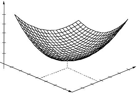
182 |
Wiener Filters |
E [e2]
w |
w |
optimal |
1 |
w
0
Figure 6.2 Mean square error surface for a two-tap FIR filter.
bowl-shaped surface, with a single minimum point, as illustrated in Figure 6.2. The least mean square error point corresponds to the minimum error power. At this optimal operating point the mean square error surface has zero gradient. From Equation (6.5), the gradient of the mean square error function with respect to the filter coefficient vector is given by
|
∂ |
E[e2 (m)]= − 2E[x(m) y(m)]+ 2wT E[ y(m) yT (m)] |
|
||||||||||
|
|
|
|||||||||||
|
∂ w |
|
|
|
|
|
|
|
|
|
(6.7) |
||
|
|
|
|
|
= − 2 ryx + 2wT Ryy |
|
|
||||||
|
|
|
|
|
|
|
|
||||||
where the gradient vector is defined as |
|
|
|
||||||||||
|
|
|
∂ |
|
∂ |
∂ |
∂ |
∂ T |
|
||||
|
|
|
|
= |
|
, |
|
, |
|
, , |
|
|
(6.8) |
|
|
|
∂ w |
|
|
|
|
||||||
|
|
|
|
∂ w0 |
∂ w1 |
∂ w2 |
∂ wP−1 |
|
|||||
The minimum mean square error Wiener filter is obtained by setting Equation (6.7) to zero:
Ryy w = ryx |
(6.9) |
Least Square Error Estimation |
183 |
or, equivalently, |
|
w = R−yy1 ryx |
(6.10) |
In an expanded form, the Wiener filter solution Equation (6.10) can be written as
|
w |
|
|
|
r |
yy |
(0) |
|
0 |
|
|
|
|
|
|
|
w1 |
|
|
|
ryy (1) |
||
|
w2 |
|
= |
|
ryy (2) |
||
|
|
|
|||||
|
|
|
|
|
|
|
|
|
|
|
|
|
|
|
|
wP−1 |
|
|
ryy (P − 1) |
||||
ryy (1) ryy (0) ryy (1)
ryy (P − 2)
ryy (2)
ryy (1)
ryy (0)
ryy (P − 3)
ryy (P − |
1) |
−1 |
|
r |
yx |
(0) |
|
||||
|
|
|
|
|
|||||||
ryy (P − |
|
|
|
|
ryx (1) |
|
|||||
2) |
|
||||||||||
ryy (P − |
3) |
|
|
|
ryx (2) |
|
|||||
|
|
|
|||||||||
|
|
||||||||||
|
|
|
|
|
|
|
|
|
|
||
|
|
|
|
|
|
||||||
|
r |
|
|
|
|
|
|
||||
|
yy |
(0) |
|
|
|
|
|
|
|
||
|
|
|
|
|
|
ryx (P − 1) |
|
||||
(6.11)
From Equation (6.11), the calculation of the Wiener filter coefficients requires the autocorrelation matrix of the input signal and the crosscorrelation vector of the input and the desired signals.
In statistical signal processing theory, the correlation values of a random process are obtained as the averages taken across the ensemble of different realisations of the process as described in Chapter 3. However in many practical situations there are only one or two finite-duration realisations of the signals x(m) and y(m). In such cases, assuming the signals are correlation-ergodic, we can use time averages instead of ensemble averages. For a signal record of length N samples, the time-averaged correlation values are computed as
|
1 |
N −1 |
|
|
ryy (k) = |
∑ y(m) y(m + k) |
(6.12) |
||
|
||||
|
N m=0 |
|
||
Note from Equation (6.11) that the autocorrelation matrix Ryy has a highly regular Toeplitz structure. A Toeplitz matrix has constant elements along the left–right diagonals of the matrix. Furthermore, the correlation matrix is also symmetric about the main diagonal elements. There are a number of efficient methods for solving the linear matrix Equation (6.11), including the Cholesky decomposition, the singular value decomposition and the QR decomposition methods.
184
6.2 Block-Data Formulation of the Wiener Filter
Wiener Filters
In this section we consider an alternative formulation of a Wiener filter for a block of N samples of the input signal [y(0), y(1), ..., y(N–1)] and the desired signal [x(0), x(1), ..., x(N–1)]. The set of N linear equations describing the Wiener filter input/output relation can be written in matrix form as
|
xˆ(0) |
|
|
y(0) |
y(−1) |
y(−2) |
|
y(2 − P) |
|
xˆ(1) |
|
|
y(1) |
y(0) |
y(−1) |
|
y(3 − P) |
|
|
|
||||||
|
xˆ(2) |
|
|
y(2) |
y(1) |
y(0) |
|
y(4 − P) |
|
|
|
= |
|
|
|
|
|
|
|
|
|
|
|
|
|
|
|
|
|
|
|
y(N − 3) y(N − 4) y(N − P) |
|||
xˆ(N − 2) |
|
y(N − 2) |
||||||
|
|
|
|
|
y(N − 2) y(N − 3) y(N + 1− P) |
|||
xˆ(N −1) |
|
y(N − 1) |
||||||
y(1− P) y(2 − P) y(3 − P)
y(N −1− P) y(N − P)
|
w0 |
|
w1 |
|
|
|
w2 |
|
|
|
|
|
|
wP−2
wP−1
|
(6.13) |
Equation (6.13) can be rewritten in compact matrix notation as |
|
ˆ |
(6.14) |
x =Y w |
The Wiener filter error is the difference between the desired signal and the
filter output defined as
e = x − xˆ
(6.15)
= x − Yw
The energy of the error vector, that is the sum of the squared elements of the error vector, is given by the inner vector product as
eTe = (x−Y w)T (x−Y w) |
(6.16) |
|
= xT x− xTYw− wTY T x + wTY TYw |
||
|
The gradient of the squared error function with respect to the Wiener filter coefficients is obtained by differentiating Equation (6.16):
∂ |
e |
T |
e |
= − 2xTY + 2wTY TY |
(6.17) |
|
|
||||
|
|
|
|
||
∂ w |
|
||||
Block-Data Formulation |
185 |
The Wiener filter coefficients are obtained by setting the gradient of the squared error function of Equation (6.17) to zero, this yields
(Y TY )w =Y T x |
(6.18) |
or |
|
−1 |
(6.19) |
w = (Y TY ) Y T x |
Note that the matrix YTY is a time-averaged estimate of the autocorrelation matrix of the filter input signal Ryy, and that the vector YTx is a timeaveraged estimate of rxy the cross-correlation vector of the input and the desired signals. Theoretically, the Wiener filter is obtained from minimisation of the squared error across the ensemble of different realisations of a process as described in the previous section. For a correlation-ergodic process, as the signal length N approaches infinity the block-data Wiener filter of Equation (6.19) approaches the Wiener filter of Equation (6.10):
lim |
−1 |
|
= R−1r |
|
|
w=(Y TY ) |
Y T x |
(6.20) |
|||
|
|
|
|
yy xy |
|
N →∞ |
|
|
|
|
|
Since the least square error method described in this section requires a block of N samples of the input and the desired signals, it is also referred to as the block least square (BLS) error estimation method. The block estimation method is appropriate for processing of signals that can be considered as time-invariant over the duration of the block.
6.2.1 QR Decomposition of the Least Square Error Equation
An efficient and robust method for solving the least square error Equation (6.19) is the QR decomposition (QRD) method. In this method, the N P signal matrix Y is decomposed into the product of an N N orthonormal matrix Q and a P P upper-triangular matrix R as
R |
|
|
|
QY = |
|
|
(6.21) |
|
0 |
||
186 |
Wiener Filters |
where 0 is the (N − P) P null matrix, |
QTQ= QQT = I , and the upper- |
triangular matrix R is of the form |
|
|
r |
r |
r |
r |
|
|
|
00 |
01 |
02 |
03 |
|
|
0 |
r11 |
r12 |
r13 |
|
|
0 |
0 |
r |
r |
R = |
|
|
|
22 |
23 |
0 |
0 |
0 |
r |
||
|
|
|
|
|
33 |
|
|
|
|
|
|
|
|
||||
|
|
0 |
0 |
0 |
0 |
|
|
||||
|
r |
|
|
|
0P−1 |
|
|
|
r1P−1 |
|
|
|
|
|
|
|
r2P−1 |
|
|
|
r3P−1 |
|
(6.22) |
|
|
|
|
|
|
||
|
|
|
|
|
rP−1P−1 |
|
|
Substitution of Equation (6.21) in Equation (6.18) yields
R |
T |
|
R |
|
R |
T |
(6.23) |
|
|
QQT |
w= |
Qx |
|||
0 |
|
|
0 |
|
0 |
|
|
From Equation (6.23) we have |
|
|
|
|
|
||
|
|
R |
|
|
|
|
|
|
|
|
w=Qx |
|
(6.24) |
||
|
|
|
0 |
|
|
|
|
From Equation (6.24) we have |
|
|
|
|
|
||
|
|
R w = xQ |
|
|
(6.25) |
||
where the vector xQ on the right hand side of Equation (6.25) is composed of the first P elements of the product Qx. Since the matrix R is uppertriangular, the coefficients of the least square error filter can be obtained easily through a process of back substitution from Equation (6.25), starting with the coefficient wP−1 =xQ (P − 1) / rP−1P−1 .
The main computational steps in the QR decomposition are the determination of the orthonormal matrix Q and of the upper triangular matrix R. The decomposition of a matrix into QR matrices can be achieved using a number of methods, including the Gram-Schmidt orthogonalisation method, the Householder method and the Givens rotation method.
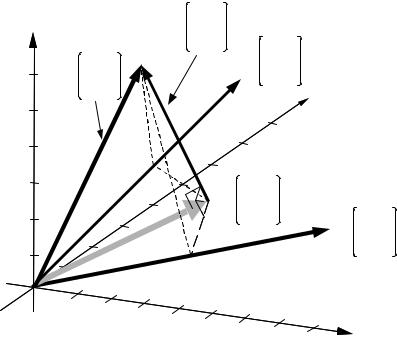
Interpretation of Wiener Filters as Projection in Vector Space |
187 |
|
Error |
|
|
Clean |
signal e(m) |
|
Noisy |
e = e(m–1) |
|
||
signal |
e(m–2) |
y(m) |
signal |
|
|
|
|
x(m) |
y = |
y(m–1) |
|
x = x(m–1) |
2 |
y(m–2) |
|
|
|
||
x(m–2) |
|
|
|
|
^ |
Noisy |
|
signal |
|
^ |
x(m) |
|
^ |
|
|
x = |
x(m–1) |
|
|
^ |
y(m–1) |
|
x(m–2) |
|
|
y = |
y(m–2) |
|
1 |
y(m–3) |
|
|
Figure 6.3 The least square error projection of a desired signal vector x onto a plane containing the input signal vectors y1 and y2 is the perpendicular projection
of x shown as the shaded vector.
6.3 Interpretation of Wiener Filters as Projection in Vector Space
In this section, we consider an alternative formulation of Wiener filters where the least square error estimate is visualized as the perpendicular minimum distance projection of the desired signal vector onto the vector space of the input signal. A vector space is the collection of an infinite number of vectors that can be obtained from linear combinations of a number of independent vectors.
In order to develop a vector space interpretation of the least square error estimation problem, we rewrite the matrix Equation (6.11) and express the filter output vector xˆ as a linear weighted combination of the column vectors of the input signal matrix as