

Литература / Advanced Digital Signal Processing and Noise Reduction (Saeed V. Vaseghi) / 06 - Wiener filters
.pdf188 |
|
|
|
|
|
|
|
|
|
|
|
|
|
|
|
|
|
|
|
Wiener Filters |
||
|
xˆ(0) |
|
|
|
|
|
y(0) |
|
|
|
|
|
|
y(−1) |
|
|
|
|
y(1 − P) |
|
||
|
xˆ(1) |
|
|
|
|
|
y(1) |
|
|
|
|
|
|
y(0) |
|
|
|
|
y(2 − P) |
|
||
|
|
|
|
|
|
|
|
|
|
|
|
|
|
|
|
|
||||||
|
xˆ(2) |
|
= w |
|
|
|
y(2) |
|
|
|
+ w |
|
y(1) |
|
+ + w |
|
|
y(3 − P) |
|
|||
|
|
|
|
|
|
|
|
|
|
|
|
|
|
|
P−1 |
|
|
|
||||
|
|
|
|
0 |
|
|
|
|
|
|
|
1 |
|
|
|
|
|
|
|
|
||
|
|
|
|
|
|
|
|
|
|
|
|
|
|
|
|
|
|
|
|
|
|
|
xˆ(N − 2) |
|
|
|
|
y(N − |
2) |
|
|
|
y(N − 3) |
|
|
|
y(N − 1 − P) |
||||||||
|
|
|
|
|
|
|
|
|
|
|
|
|
|
|
|
|
|
|
|
|
|
|
xˆ(N − 1) |
|
|
|
|
y(N − |
1) |
|
|
y(N − 2) |
|
|
|
|
y(N − P) |
||||||||
|
|
|
|
|
|
|
|
|
|
|
|
|
|
|
|
|
|
|
|
|
|
(6.26) |
In compact notation, Equation (6.26) may be written as |
|
|
|
|||||||||||||||||||
|
|
|
ˆ |
|
= |
w0 y0 |
+ |
w1 |
y1 |
+ + |
wP−1 yP−1 |
|
|
|
(6.27) |
|||||||
|
|
|
x |
|
|
|
|
|
|
|
|
|
|
|||||||||
In Equation (6.27) the signal estimate xˆ is a linear combination of P basis vectors [y0, y1, . . ., yP–1], and hence it can be said that the estimate xˆ is in the vector subspace formed by the input signal vectors [y0, y1, . . ., yP–1].
In general, the P N-dimensional input signal vectors [y0, y1, . . ., yP–1] in Equation (6.27) define the basis vectors for a subspace in an N- dimensional signal space. If P, the number of basis vectors, is equal to N, the vector dimension, then the subspace defined by the input signal vectors encompasses the entire N-dimensional signal space and includes the desired signal vector x. In this case, the signal estimate xˆ = x and the estimation error is zero. However, in practice, N>P, and the signal space defined by the P input signal vectors of Equation (6.27) is only a subspace of the N- dimensional signal space. In this case, the estimation error is zero only if the desired signal x happens to be in the subspace of the input signal, otherwise the best estimate of x is the perpendicular projection of the vector x onto the vector space of the input signal [y0, y1, . . ., yP–1]., as explained in the following example.
Example 6.1 Figure 6.3 illustrates a vector space interpretation of a simple least square error estimation problem, where yT=[y(2), y(1), y(0), y(– 1)] is the input signal, xT=[x(2), x(1), x(0)] is the desired signal and wT=[w0, w1] is the filter coefficient vector. As in Equation (6.26), the filter output can be written as
Analysis of the Least Mean Square Error Signal |
|
|
|
|
|
189 |
|||||||
xˆ(2) |
|
|
y(2) |
|
|
|
|
y(1) |
|
|
|
||
|
|
= w0 |
|
|
+ |
|
|
|
|
|
|
|
|
xˆ(1) |
|
y(1) |
|
w1 |
y(0) |
|
|
(6.28) |
|||||
ˆ |
|
|
|
|
|
|
|
|
− |
|
|
|
|
x(0) |
|
|
y(0) |
|
|
|
y( |
|
1) |
|
|
|
|
In Equation (6.28), the |
input signal |
vectors |
yT =[y(2), |
y(1), |
y(0)] and |
||||||||
|
|
|
|
|
|
|
|
|
|
|
1 |
|
|
y2T =[y(1), y(0), y(−1)] are 3-dimensional vectors. The subspace defined by the linear combinations of the two input vectors [y1, y2] is a 2-dimensional plane in a 3-dimensional signal space. The filter output is a linear combination of y1 and y2, and hence it is confined to the plane containing these two vectors. The least square error estimate of x is the orthogonal projection of x on the plane of [y1, y2] as shown by the shaded vector xˆ . If the desired vector happens to be in the plane defined by the vectors y1 and y2 then the estimation error will be zero, otherwise the estimation error will be the perpendicular distance of x from the plane containing y1 and y2.
6.4 Analysis of the Least Mean Square Error Signal
The optimality criterion in the formulation of the Wiener filter is the least mean square distance between the filter output and the desired signal. In this section, the variance of the filter error signal is analysed. Substituting the Wiener equation Ryyw=ryx in Equation (6.5) gives the least mean square error:
E[e2 (m)] = rxx (0) − wT ryx |
|
|
|
= r (0) −wT R |
yy |
w |
(6.29) |
|
|||
xx |
|
|
|
Now, for zero-mean signals, it is easy to show that in Equation (6.29) the term wTRyyw is the variance of the Wiener filter output xˆ(m) :
2 |
= |
ˆ |
2 |
(m)] |
= |
w |
T |
Ryy w |
(6.30) |
σ xˆ |
|
E[x |
|
|
|
Therefore Equation (6.29) may be written as
σ e2 = σ x2 −σ x2ˆ |
(6.31) |
190 |
|
|
|
|
|
|
|
|
Wiener Filters |
2 |
=E[x |
2 |
2 |
ˆ |
2 |
2 |
=E[e |
2 |
(m)] are the variances |
where σ x |
|
(m)],σ xˆ |
=E[x |
|
(m)] and σ e |
|
of the desired signal, the filter estimate of the desired signal and the error signal respectively. In general, the filter input y(m) is composed of a signal component xc(m) and a random noise n(m):
y(m)= xc (m)+n(m) |
(6.32) |
where the signal xc(m) is the part of the observation that is correlated with the desired signal x(m), and it is this part of the input signal that may be transformable through a Wiener filter to the desired signal. Using Equation (6.32) the Wiener filter error may be decomposed into two distinct components:
|
P |
|
|
e(m) = x(m)− ∑ wk y(m − k) |
|
|
|
|
k=0 |
|
|
|
P |
|
P |
= x(m) − ∑wk xc (m − k) |
− ∑ wk n(m − k) |
||
|
k=0 |
|
k =0 |
or
e(m) =ex (m)+en (m)
(6.33)
(6.34)
where ex(m) is the difference between the desired signal x(m) and the output of the filter in response to the input signal component xc(m), i.e.
P−1 |
|
ex (m)= x(m)− ∑ wk xc (m − k) |
(6.35) |
k =0
and en(m) is the error in the output due to the presence of noise n(m) in the input signal:
P−1
en (m)=− ∑wk n(m − k)
k=0
The variance of filter error can be rewritten as
σ 2 =σ 2 +σ 2
e ex en
(6.36)
(6.37)
Formulation of Wiener Filter in the Frequency Domain |
191 |
Note that in Equation (6.34), ex(m) is that part of the signal that cannot be recovered by the Wiener filter, and represents distortion in the signal output, and en(m) is that part of the noise that cannot be blocked by the Wiener filter. Ideally, ex(m)=0 and en(m)=0, but this ideal situation is possible only if the following conditions are satisfied:
(a)The spectra of the signal and the noise are separable by a linear filter.
(b)The signal component of the input, that is xc(m), is linearly transformable to x(m).
(c)The filter length P is sufficiently large. The issue of signal and noise separability is addressed in Section 6.6.
6.5Formulation of Wiener Filters in the Frequency Domain
In the frequency domain, the Wiener filter output ˆ is the product of the
X( f ) input signal Y(f) and the filter frequency response W(f):
ˆ |
(6.38) |
X ( f ) =W ( f )Y ( f ) |
The estimation error signal E(f) is defined as the difference between the
desired signal X(f) and the filter output ˆ ,
X( f )
= − ˆ
E( f ) X ( f ) X ( f )
= X ( f ) −W ( f )Y ( f )
and the mean square error at a frequency f is given by
E |
|
E( f ) |
|
2 |
=E[(X ( f )−W ( f )Y ( f ))* (X ( f )−W ( f )Y ( f ))] |
|
|
||||
|
|
|
|
|
|
|
|
|
|
(6.39)
(6.40)
where E[·] is the expectation function, and the symbol * denotes the complex conjugate. Note from Parseval’s theorem that the mean square error in time and frequency domains are related by
192 |
|
|
|
|
|
Wiener Filters |
|
|
|
|
|
|
|
N −1 |
1/ 2 |
|
|
|
||
∑e2 (m) = |
∫ |
|
E( f ) |
|
2 df |
(6.41) |
|
|
|||||
m=0 |
−1/ 2 |
|
||||
To obtain the least mean square error filter we set the complex derivative of Equation (6.40) with respect to filter W(f) to zero
∂ E [| E( f ) |2 ] = 2W ( f )P |
( f ) − 2P ( f ) = 0 |
(6.42) |
|
∂W ( f ) |
YY |
XY |
|
|
|
|
|
where PYY(f)=E[Y(f)Y*(f)] and PXY(f)=E[X(f)Y*(f)] are the power spectrum of Y(f), and the cross-power spectrum of Y(f) and X(f) respectively. From Equation (6.42), the least mean square error Wiener filter in the frequency domain is given as
W ( f )= |
PXY ( f ) |
(6.43) |
|
PYY ( f ) |
|||
|
|
Alternatively, the frequency-domain Wiener filter Equation (6.43) can be obtained from the Fourier transform of the time-domain Wiener Equation (6.9):
P−1 |
− jωm = ∑ ryx (n)e− jωm |
|
∑ ∑ wk ryy (m − k)e |
(6.44) |
|
m k =0 |
m |
|
From the Wiener–Khinchine relation, the correlation and power-spectral functions are Fourier transform pairs. Using this relation, and the Fourier transform property that convolution in time is equivalent to multiplication in frequency, it is easy to show that the Wiener filter is given by Equation (6.43).
6.6 Some Applications of Wiener Filters
In this section, we consider some applications of the Wiener filter in reducing broadband additive noise, in time-alignment of signals in multichannel or multisensor systems, and in channel equalisation.
Some Applications of Wiener Filters |
193 |
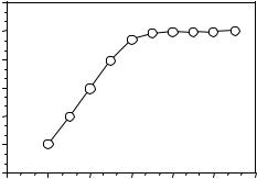
20 log W(f)
20
0
-20
-40
-60
-80
-100
-60 |
-40 |
-20 |
0 |
20 |
40 |
60 |
SNR (dB)
Figure 6.4 Variation of the gain of Wiener filter frequency response with SNR.
6.6.1 Wiener Filter for Additive Noise Reduction
Consider a signal x(m) observed in a broadband additive noise n(m)., and model as
y(m) = x(m) + n(m) |
(6.45) |
Assuming that the signal and the noise are uncorrelated, it follows that the autocorrelation matrix of the noisy signal is the sum of the autocorrelation matrix of the signal x(m) and the noise n(m):
Ryy = Rxx + Rnn |
(6.46) |
and we can also write |
|
rxy = rxx |
(6.47) |
where Ryy, Rxx and Rnn are the autocorrelation matrices of the noisy signal, the noise-free signal and the noise respectively, and rxy is the crosscorrelation vector of the noisy signal and the noise-free signal. Substitution of Equations (6.46) and (6.47) in the Wiener filter, Equation (6.10), yields
w =(Rxx + Rnn )−1 rxx |
(6.48) |
Equation (6.48) is the optimal linear filter for the removal of additive noise. In the following, a study of the frequency response of the Wiener filter provides useful insight into the operation of the Wiener filter. In the frequency domain, the noisy signal Y(f) is given by
194 |
Wiener Filters |
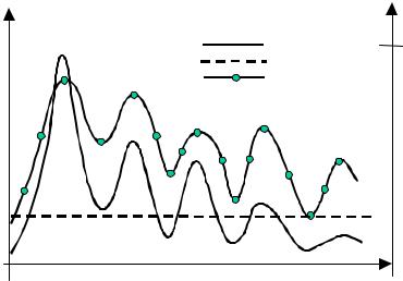
Signal and noise magnitudespectrum |
Signal |
1.0 |
Noise |
Wiener filter magnitude W(f) |
|
Wiener filter |
||
|
||
|
|
0.0 |
Frequency |
(f) |
|
Figure 6.5 Illustration of the variation of Wiener frequency response with signal spectrum for additive white noise. The Wiener filter response broadly follows the
signal spectrum. |
|
Y ( f )= X ( f )+ N ( f ) |
(6.49) |
where X(f) and N(f) are the signal and noise spectra. For a signal observed in additive random noise, the frequency-domain Wiener filter is obtained as
W ( f ) = |
PXX |
( f ) |
|
|
|
(6.50) |
|
|
|
||
|
PXX ( f ) + PNN ( f ) |
||
where PXX(f) and PNN(f) are the signal and noise power spectra. Dividing the numerator and the denominator of Equation (6.50) by the noise power spectra PNN(f) and substituting the variable SNR(f)=PXX(f)/PNN(f) yields
W ( f ) = |
SNR( f ) |
|
(6.51) |
|
SNR( f ) +1 |
||||
|
|
|||
where SNR is a signal-to-noise ratio measure. Note that the variable, SNR(f) is expressed in terms of the power-spectral ratio, and not in the more usual terms of log power ratio. Therefore SNR(f)=0 corresponds to − ∞ dB.
From Equation (6.51), the following interpretation of the Wiener filter frequency response W(f) in terms of the signal-to-noise ratio can be
Some Applications of Wiener Filters |
|
195 |
|
Magnitude |
|
Magnitude |
Signal |
|
|
Noise |
|
|
|
|
|
|
spectra |
Overlapped spectra |
|
|
Separable |
|
|
(a) |
Frequency |
(b) |
Frequency |
Figure 6.6 Illustration of separability: (a) The signal and noise spectra do not overlap, and the signal can be recovered by a low-pass filter; (b) the signal and noise spectra overlap, and the noise can be reduced but not completely removed.
deduced. For additive noise, the Wiener filter frequency response is a real positive number in the range 0≤ W ( f ) ≤ 1. Now consider the two limiting cases of (a) a noise-free signal SNR( f ) = ∞ and (b) an extremely noisy signal SNR(f)=0. At very high SNR, W ( f ) ≈1, and the filter applies little or no attenuation to the noise-free frequency component. At the other extreme, when SNR(f)=0, W(f)=0. Therefore, for additive noise, the Wiener filter attenuates each frequency component in proportion to an estimate of the signal to noise ratio. Figure 6.4 shows the variation of the Wiener filter response W(f), with the signal-to-noise ratio SNR(f).
An alternative illustration of the variations of the Wiener filter frequency response with SNR(f) is shown in Figure 6.5. It illustrates the similarity between the Wiener filter frequency response and the signal spectrum for the case of an additive white noise disturbance. Note that at a spectral peak of the signal spectrum, where the SNR(f) is relatively high, the Wiener filter frequency response is also high, and the filter applies little attenuation. At a signal trough, the signal-to-noise ratio is low, and so is the Wiener filter response. Hence, for additive white noise, the Wiener filter response broadly follows the signal spectrum.
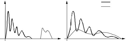
6.6.2 Wiener Filter and the Separability of Signal and Noise
A signal is completely recoverable from noise if the spectra of the signal and the noise do not overlap. An example of a noisy signal with separable signal and noise spectra is shown in Figure 6.6(a). In this case, the signal
196 |
Wiener Filters |
and the noise occupy different parts of the frequency spectrum, and can be separated with a low-pass, or a high-pass, filter. Figure 6.6(b) illustrates a more common example of a signal and noise process with overlapping spectra. For this case, it is not possible to completely separate the signal from the noise. However, the effects of the noise can be reduced by using a Wiener filter that attenuates each noisy signal frequency in proportion to an estimate of the signal-to-noise ratio as described by Equation (6.51).
6.6.3 The Square-Root Wiener Filter
In the frequency domain, the Wiener filter output ˆ is the product of the
X( f )
input frequency X(f) and the filter response W(f) as expressed in Equation (6.38). Taking the expectation of the squared magnitude of both sides of Equation (6.38) yields the power spectrum of the filtered signal as
ˆ |
2 |
] = |
|
|
W ( f ) |
|
2 |
E[| |
Y ( f ) | |
2 |
] |
|
|
|
|
||||||||||
E[| X ( f ) | |
|
|
|
|
|
|
||||||
|
|
= |
|
W ( f ) |
|
|
2 P |
( f ) |
|
(6.52) |
||
|
|
|
|
|
|
|
||||||
|
|
|
|
|
|
|
|
|
YY |
|
|
|
Substitution of W(f) from Equation (6.43) in Equation (6.52) yields
ˆ |
|
|
2 |
|
P2 |
( f ) |
|
||||
|
|
] = |
XY |
|
|
|
|
|
|||
E[| X ( f ) | |
|
|
|
|
|
|
|
(6.53) |
|||
|
|
PYY ( f ) |
|||||||||
|
|
|
|
|
|
|
|||||
Now, for a signal observed in an uncorrelated additive noise we have |
|
||||||||||
PYY ( f )=PXX ( f )+PNN ( f ) |
(6.54) |
||||||||||
and |
|
|
|
|
|
|
|
|
|
|
|
PXY ( f )=PXX ( f ) |
(6.55) |
||||||||||
Substitution of Equations (6.54) and (6.55) in Equation (6.53) yields |
|
||||||||||
ˆ |
2 |
|
|
|
|
P2 |
|
( f ) |
|
||
]= |
|
|
XX |
|
|
|
|
||||
E[| X ( f ) | |
|
|
|
|
|
|
|
|
(6.56) |
||
|
PXX ( f ) |
+ PNN ( f ) |
|||||||||
|
|
|
|
|
|||||||
Now, in Equation (6.38) if instead of the Wiener filter, the square root of the Wiener filter magnitude frequency response is used, the result is

Some Applications of Wiener Filters |
|
|
|
197 |
||
ˆ |
|
W ( f ) |
|
1/ 2 |
Y ( f ) |
(6.57) |
|
|
|||||
X ( f ) = |
|
|
|
|||
and the power spectrum of the signal, filtered by the square-root Wiener filter, is given by
ˆ |
2 |
|
|
1/ 2 |
2 |
|
|
|
2 |
|
PXY ( f ) |
|
|
|
|
|
|
|
|
|
|||||||
E [| X ( f ) | |
|
]= [ |
W ( f ) |
|
] |
E[ |
Y ( f ) |
|
] = |
|
PYY ( f ) =PXY |
( f ) |
|
|
|
|
P ( f ) |
||||||||||
|
|
|
|
|
|
|
|
|
|
||||
|
|
|
|
|
|
|
|
|
|
|
YY |
|
|
Now, for uncorrelated signal and noise Equation (6.58) becomes |
|
||||||||||||
|
|
|
|
ˆ |
|
|
2 |
]= PXX ( f ) |
|
|
|||
|
|
|
E[| X ( f ) | |
|
|
|
|||||||
(6.58)
(6.59)
Thus, for additive noise the power spectrum of the output of the square-root Wiener filter is the same as the power spectrum of the desired signal.
6.6.4 Wiener Channel Equaliser
Communication channel distortions may be modelled by a combination of a linear filter and an additive random noise source as shown in Figure 6.7. The input/output signals of a linear time invariant channel can be modelled as
P−1 |
|
y(m)= ∑hk x(m − k)+n(m) |
(6.60) |
k=0
where x(m) and y(m) are the transmitted and received signals, [hk] is the impulse response of a linear filter model of the channel, and n(m) models the channel noise. In the frequency domain Equation (6.60) becomes
Y ( f )= X ( f )H ( f )+ N ( f ) |
(6.61) |
where X(f), Y(f), H(f) and N(f) are the signal, noisy signal, channel and noise spectra respectively. To remove the channel distortions, the receiver is followed by an equaliser. The equaliser input is the distorted channel output, and the desired signal is the channel input. Using Equation (6.43) it is easy to show that the Wiener equaliser in the frequency domain is given by