

Литература / Advanced Digital Signal Processing and Noise Reduction (Saeed V. Vaseghi) / 11 - Spectral subtraction
.pdfAdvanced Digital Signal Processing and Noise Reduction, Second Edition.
Saeed V. Vaseghi
Copyright © 2000 John Wiley & Sons Ltd
ISBNs: 0-471-62692-9 (Hardback): 0-470-84162-1 (Electronic)
Noise-free signal space |
Noisy signal space |
After subtraction of |
fh |
fh |
the noise mean |
fh |
11
fl |
fl |
|
fl |
SPECTRAL SUBTRACTION
11.1Spectral Subtraction
11.2Processing Distortions
11.3Non-Linear Spectral Subtraction
11.4Implementation of Spectral Subtraction
11.5Summary
Spectral subtraction is a method for restoration of the power spectrum or the magnitude spectrum of a signal observed in additive noise, through subtraction of an estimate of the average noise spectrum from the noisy signal spectrum. The noise spectrum is usually estimated, and
updated, from the periods when the signal is absent and only the noise is present. The assumption is that the noise is a stationary or a slowly varying process, and that the noise spectrum does not change significantly inbetween the update periods. For restoration of time-domain signals, an estimate of the instantaneous magnitude spectrum is combined with the phase of the noisy signal, and then transformed via an inverse discrete Fourier transform to the time domain. In terms of computational complexity, spectral subtraction is relatively inexpensive. However, owing to random variations of noise, spectral subtraction can result in negative estimates of the short-time magnitude or power spectrum. The magnitude and power spectrum are non-negative variables, and any negative estimates of these variables should be mapped into non-negative values. This nonlinear rectification process distorts the distribution of the restored signal. The processing distortion becomes more noticeable as the signal-to-noise ratio decreases. In this chapter, we study spectral subtraction, and the different methods of reducing and removing the processing distortions.

334
11.1 Spectral Subtraction
Spectral Subtraction
In applications where, in addition to the noisy signal, the noise is accessible on a separate channel, it may be possible to retrieve the signal by subtracting an estimate of the noise from the noisy signal. For example, the adaptive noise canceller of Section 1.3.1 takes as the inputs the noise and the noisy signal, and outputs an estimate of the clean signal. However, in many applications, such as at the receiver of a noisy communication channel, the only signal that is available is the noisy signal. In these situations, it is not possible to cancel out the random noise, but it may be possible to reduce the average effects of the noise on the signal spectrum. The effect of additive noise on the magnitude spectrum of a signal is to increase the mean and the variance of the spectrum as illustrated in Figure 11.1. The increase in the variance of the signal spectrum results from the random fluctuations of the noise, and cannot be cancelled out. The increase in the mean of the signal spectrum can be removed by subtraction of an estimate of the mean of the noise spectrum from the noisy signal spectrum. The noisy signal model in the time domain is given by
|
|
|
|
|
y(m)= x(m) |
|
6 x10⁵ |
|
|
|
|
|
|
4 |
|
|
|
|
|
|
2 |
|
|
|
|
|
|
0 |
|
|
|
|
|
|
-2 |
|
|
|
|
|
|
-4 |
|
|
|
|
|
|
-6 |
200 |
400 |
600 |
800 |
1000 |
1200 |
0 |
||||||
20 |
|
|
|
|
|
|
15 |
|
|
|
|
|
|
10 |
|
|
|
|
|
|
5 |
|
|
|
|
|
|
0 |
|
|
|
|
|
|
0 |
|
50 |
100 |
150 |
200 |
250 |
+ n(m) |
|
|
|
|
(11.1) |
|
6 x10⁵ |
|
|
|
|
|
|
4 |
|
|
|
|
|
|
2 |
|
|
|
|
|
|
0 |
|
|
|
|
|
|
-2 |
|
|
|
|
|
|
-4 |
|
|
|
|
|
|
-6 |
200 |
400 |
600 |
800 |
1000 |
1200 |
0 |
||||||
20 |
|
|
|
|
|
|
15 |
|
|
|
|
|
|
10 |
|
|
|
|
|
|
5 |
|
|
|
|
|
|
0 |
50 |
|
100 |
150 |
200 |
250 |
0 |
|
|||||
Figure 11.1 Illustrations of the effect of noise on a signal in the time and the frequency domains.

Spectral Subtraction |
335 |
where y(m), x(m) and n(m) are the signal, the additive noise and the noisy signal respectively, and m is the discrete time index. In the frequency domain, the noisy signal model of Equation (11.1) is expressed as
Y ( f )= X( f )+ N( f ) |
(11.2) |
where Y(f), X(f) and N(f) are the Fourier transforms of the noisy signal y(m), the original signal x(m) and the noise n(m) respectively, and f is the frequency variable. In spectral subtraction, the incoming signal x(m) is buffered and divided into segments of N samples length. Each segment is windowed, using a Hanning or a Hamming window, and then transformed via discrete Fourier transform (DFT) to N spectral samples. The windows alleviate the effects of the discontinuities at the endpoints of each segment. The windowed signal is given by
yw (m) = w(m)y(m) |
|
= w(m)[x(m)+ n(m)] |
(11.3) |
= xw(m)+ nw(m) |
|
The windowing operation can be expressed in the frequency domain as
Yw ( f )=W ( f ) *Y ( f ) (11.4)
= X w ( f )+Nw ( f )
where the operator * denotes convolution. Throughout this chapter, it is assumed that the signals are windowed, and hence for simplicity we drop the use of the subscript w for windowed signals.
Figure 11.2 illustrates a block diagram configuration of the spectral subtraction method. A more detailed implementation is described in Section 11.4. The equation describing spectral subtraction may be expressed as
|
|
|
ˆ |
|
b |
= |
|
Y ( f ) |
|
b |
−α |
|
|
N( f ) |
|
b |
(11.5) |
||
|
|
|
|
|
|
|
|
||||||||||||
|
|
|
X ( f ) |
|
|
|
|
|
|
|
|
||||||||
ˆ |
b |
is an estimate of the original signal spectrum| X ( f ) | |
b |
and |
|||||||||||||||
where | X ( f ) | |
|
|
|||||||||||||||||
| N ( f ) |b is the time-averaged noise spectra. It is assumed that the noise is a wide-sense stationary random process. For magnitude spectral subtraction, the exponent b=1, and for power spectral subtraction, b=2. The parameter α
336 |
|
|
|
Spectral Subtraction |
y(m) |
Y(f) |
Post |
ˆ |
xˆ(m) |
X( f ) |
||||
|
DFT |
subtraction |
|
IDFT |
|
|
processing |
|
|
Noise estimate
Figure 11.2 A block diagram illustration of spectral subtraction.
in Equation (11.5) controls the amount of noise subtracted from the noisy signal. For full noise subtraction, α=1 and for over-subtraction α>1. The time-averaged noise spectrum is obtained from the periods when the signal is absent and only the noise is present as
|
|
1 |
K −1 |
|
|
| N ( f ) |b = |
∑ | N i ( f ) |b |
(11.6) |
|||
|
|||||
|
|
K i=0 |
|
||
In Equation (11.6), |Ni(f)| is the spectrum of the ith noise frame, and it is assumed that there are K frames in a noise-only period, where K is a variable. Alternatively, the averaged noise spectrum can be obtained as the output of a first order digital low-pass filter as
| N i ( f ) |b = ρ | N i−1 ( f ) |b +(1− ρ ) | N i ( f ) |b |
(11.7) |
where the low-pass filter coefficient ρ is typically set between 0.85 and 0.99. For restoration of a time-domain signal, the magnitude spectrum
estimate | ˆ ( ) | is combined with the phase of the noisy signal, and then
X f
transformed into the time domain via the inverse discrete Fourier transform as
N −1 |
ˆ |
jθY (k) |
− j |
2π |
km |
xˆ(m) = ∑ |
N |
||||
| X (k) | e |
|
e |
|
(11.8) |
|
k =0 |
|
|
|
|
|
where θY (k) is the phase of the noisy signal frequency Y(k). The signal restoration equation (11.8) is based on the assumption that the audible noise is mainly due to the distortion of the magnitude spectrum, and that the phase distortion is largely inaudible. Evaluations of the perceptual effects of simulated phase distortions validate this assumption.
Spectral Subtraction |
337 |
Owing to the variations of the noise spectrum, spectral subtraction may result in negative estimates of the power or the magnitude spectrum. This outcome is more probable as the signal-to-noise ratio (SNR) decreases. To avoid negative magnitude estimates the spectral subtraction output is postprocessed using a mapping function T[·] of the form
ˆ |
|
ˆ |
ˆ |
|
| X ( f ) | |
if | X ( f ) |>β | Y ( f ) | |
|
T [| X ( |
f ) |]= |
|
(11.9) |
|
fn[| Y ( f ) |] |
otherwise |
|
|
|
|
|
For example, |
we may chose |
a rule such that if the estimate |
|
ˆ |
|
(in magnitude spectrum 0.01 is equivalent to –40 dB) |
|
| X ( f ) |> 0.01| Y ( f ) | |
|||
then | ˆ ( )| should be set to some function of the noisy signal fn[Y(f)]. In its
X f
simplest form, fn[Y(f)]=noise floor, where the noise floor is a positive constant. An alternative choice is fn[|Y(f)|]=β |Y(f)|. In this case,
ˆ |
|
ˆ |
| X ( f ) | |
||
T [| X ( f ) |]= |
β | Y ( f ) | |
|
|
|
|
|
|
|
ˆ >β
if | X ( f ) | | Y ( f ) |
(11.10)
otherwise
Spectral subtraction may be implemented in the power or the magnitude spectral domains. The two methods are similar, although theoretically they result in somewhat different expected performance.
11.1.1 Power Spectrum Subtraction
The power spectrum subtraction, or squared-magnitude subtraction, is defined by the following equation:
ˆ |
2 |
= | Y ( f ) | |
2 |
− | N ( f ) | |
2 |
| X ( f ) | |
|
|
|
spectrum
(11.11)
where it is assumed that α, the subtraction factor in Equation (11.5), is unity. We denote the power spectrum by E[| X ( f ) |2 ] , the time-averaged
power spectrum by X ( f ) 2 and the instantaneous power spectrum by
X ( f ) 2 . By expanding the instantaneous power spectrum of the noisy

338 Spectral Subtraction
signal Y ( f ) 2 , and grouping the appropriate terms, Equation (11.11) may be rewritten as
ˆ |
|
|
|
|
|
|
|
|
|
|
|
|
|
|
|
2 |
=| X ( f )| |
2 |
| N ( f ) | |
2 |
− | N ( f ) | |
2 |
+ X |
* |
( f ) N ( f ) + X ( f ) N |
* |
( f ) |
||||
| X ( f ) | |
|
|
+ |
|
|
|
|
|
|||||||
|
|
|
|
|
|
|
|
|
|
|
|
||||
|
|
|
|
|
|
|
Cross products |
|
|
||||||
|
|
|
|
|
Noise variations |
|
|
|
|
|
|
|
|||
|
|
|
|
|
|
|
|
|
|
|
|
|
(11.12) |
||
Taking the expectations of both sides of Equation (11.12), and assuming that the signal and the noise are uncorrelated ergodic processes, we have
ˆ |
2 |
]=E[| X ( f ) | |
2 |
] |
(11.13) |
E[| X ( f ) | |
|
|
From Equation (11.13), the average of the estimate of the instantaneous power spectrum converges to the power spectrum of the noise-free signal. However, it must be noted that for non-stationary signals, such as speech, the objective is to recover the instantaneous or the short-time spectrum, and only a relatively small amount of averaging can be applied. Too much averaging will smear and obscure the temporal evolution of the spectral events. Note that in deriving Equation (11.13), we have not considered nonlinear rectification of the negative estimates of the squared magnitude spectrum.
11.1.2 Magnitude Spectrum Subtraction
The magnitude spectrum subtraction is defined as
|
|
|
|
|
ˆ |
|
|
|
|
|
|
|
|
− | N ( f ) | |
(11.14) |
||||||||||||
|
|
|
|
|
| X ( f ) |= | Y ( f ) | |
||||||||
|
|
|
|
|
|
|
|
|
|
|
|
||
where |
|
N ( f ) |
|
is the time-averaged |
|
magnitude spectrum |
of the noise. |
||||||
|
|
||||||||||||
Taking the expectation of Equation (11.14), we have |
|
||||||||||||
|
|
|
ˆ |
|
|
|
|
|
|
|
|||
|
|
|
|
|
|
|
|
|
|
||||
|
|
E[| X ( f ) |] =E[| Y ( f ) |]−E[| N ( f ) | ] |
|
||||||||||
|
|
|
|
|
=E[| X ( f ) + N ( f ) |]−E[ |
|
|
|
|||||
|
|
|
|
|
| N ( f ) |] |
(11.15) |
|||||||
|
|
|
|
|
≈E[| X ( f )|] |
|
|
|
|
|
|
|
|
Spectral Subtraction |
339 |
For signal restoration the magnitude estimate is combined with the phase of the noisy signal and then transformed into the time domain using Equation (11.8).
11.1.3 Spectral Subtraction Filter: Relation to Wiener Filters
The spectral subtraction equation can be expressed as the product of the noisy signal spectrum and the frequency response of a spectral subtraction filter as
ˆ |
2 |
=| Y ( f ) | |
2 |
− | N ( f ) | |
2 |
| X ( f ) | |
|
|
(11.16) |
||
|
|
|
|
|
=H ( f ) | Y ( f ) |2
where H(f), the frequency response of the spectral subtraction filter, is defined as
H ( f ) = 1 − | N ( f ) |2 | Y ( f ) |2
(11.17)
=| Y ( f ) |2 −| N ( f ) |2 | Y ( f ) |2
The spectral subtraction filter H(f) is a zero-phase filter, with its magnitude response in the range 0≥ H ( f ) ≥1. The filter acts as a SNR-dependent
attenuator. The attenuation at each frequency increases with the decreasing SNR, and conversely decreases with the increasing SNR.
The least mean square error linear filter for noise removal is the Wiener filter covered in chapter 6. Implementation of a Wiener filter requires the power spectra (or equivalently the correlation functions) of the signal and the noise process, as discussed in Chapter 6. Spectral subtraction is used as a substitute for the Wiener filter when the signal power spectrum is not available. In this section, we discuss the close relation between the Wiener filter and spectral subtraction. For restoration of a signal observed in uncorrelated additive noise, the equation describing the frequency response of the Wiener filter was derived in Chapter 6 as
W ( f ) = |
E[| Y ( f ) |2 |
]−E[| N ( f ) |2 ] |
|
|
|
(11.18) |
|
|
|
||
E[| Y ( f ) |2 ]

340 |
Spectral Subtraction |
A comparison of W(f) and H(f), from Equations (11.18) and (11.17), shows that the Wiener filter is based on the ensemble-average spectra of the signal and the noise, whereas the spectral subtraction filter uses the instantaneous spectra of the noisy signal and the time-averaged spectra of the noise. In spectral subtraction, we only have access to a single realisation of the process. However, assuming that the signal and noise are wide-sense stationary ergodic processes, we may replace the instantaneous noisy signal spectrum | Y ( f ) |2 in the spectral subtraction equation (11.18) with the time-
averaged spectrum | Y ( f ) |2 , to obtain
H ( f ) = |
| Y ( f ) |2 |
−| N ( f ) |2 |
|||
|
|
|
|
(11.19) |
|
|
|
|
|
||
| Y ( f ) |2
For an ergodic process, as the length of the time over which the signals are averaged increases, the time-averaged spectrum approaches the ensembleaveraged spectrum, and in the limit, the spectral subtraction filter of Equation (11.19) approaches the Wiener filter equation (11.18). In practice, many signals, such as speech and music, are non-stationary, and only a limited degree of beneficial time-averaging of the spectral parameters can be expected.
11.2 Processing Distortions
The main problem in spectral subtraction is the non-linear processing distortions caused by the random variations of the noise spectrum. From Equation (11.12) and the constraint that the magnitude spectrum must have a non-negative value, we may identify three sources of distortions of the instantaneous estimate of the magnitude or power spectrum as:
(a)the variations of the instantaneous noise power spectrum about the mean;
(b)the signal and noise cross-product terms;
(c)the non-linear mapping of the spectral estimates that fall below a threshold.
The same sources of distortions appear in both the magnitude and the power spectrum subtraction methods. Of the three sources of distortions listed
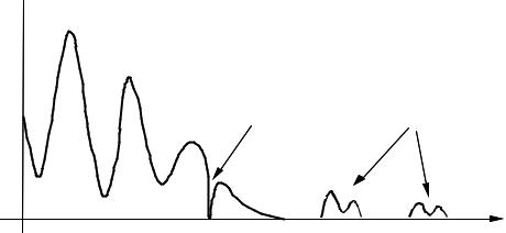
Processing Distortions |
341 |
 |y(f)|
Distortion in the form of a sharp trough in signal spectra.
Distortions in the form of Isolated “musical” noise.
f
Figure 11.3 Illustration of distortions that may result from spectral subtraction.
above, the dominant distortion is often due to the non-linear mapping of the negative, or small-valued, spectral estimates. This distortion produces a metallic sounding noise, known as “musical tone noise” due to their narrowband spectrum and the tin-like sound. The success of spectral subtraction depends on the ability of the algorithm to reduce the noise variations and to remove the processing distortions. In its worst, and not uncommon, case the residual noise can have the following two forms:
(a)a sharp trough or peak in the signal spectra;
(b)isolated narrow bands of frequencies.
In the vicinity of a high amplitude signal frequency, the noise-induced trough or peak is often masked, and made inaudible, by the high signal energy. The main cause of audible degradations is the isolated frequency components also known as musical tones or musical noise illustrated in Figure 11.3. The musical noise is characterised as short-lived narrow bands of frequencies surrounded by relatively low-level frequency components. In audio signal restoration, the distortion caused by spectral subtraction can result in a significant deterioration of the signal quality. This is particularly true at low signal-to-noise ratios. The effects of a bad implementation of subtraction algorithm can result in a signal that is of a lower perceived quality, and lower information content, than the original noisy signal.
342 |
|
Spectral Subtraction |
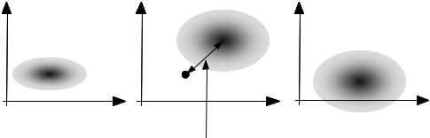
Noise-free signal space |
Noisy signal space |
After subtraction of |
fh |
fh |
the noise mean |
fh |
(a) |
fl |
(b) |
fl |
(c) |
fl |
|
|
|
|
|
|
Noise induced change in the mean
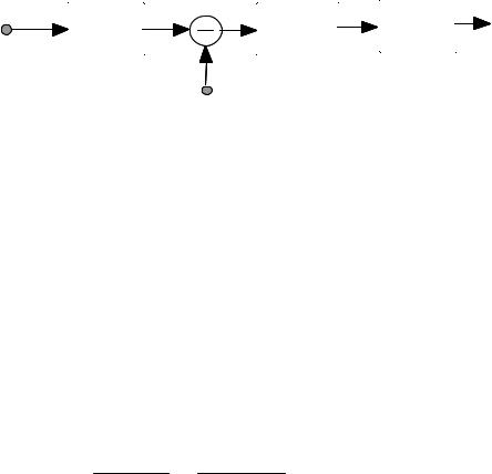
Figure 11.4 Illustration of the distorting effect of spectral subtraction on the space of the magnitude spectrum of a signal.
11.2.1 Effect of Spectral Subtraction on Signal Distribution
Figure 11.4 is an illustration of the distorting effect of spectral subtraction on the distribution of the magnitude spectrum of a signal. In this figure, we have considered the simple case where the spectrum of a signal is divided into two parts; a low-frequency band fl and a high-frequency band fh. Each point in Figure 11.4 is a plot of the high-frequency spectrum versus the lowfrequency spectrum, in a two-dimensional signal space. Figure 11.4(a) shows an assumed distribution of the spectral samples of a signal in the twodimensional magnitude–frequency space. The effect of the random noise, shown in Figure 11.4(b), is an increase in the mean and the variance of the spectrum, by an amount that depends on the mean and the variance of the magnitude spectrum of the noise. The increase in the variance constitutes an irrevocable distortion. The increase in the mean of the magnitude spectrum can be removed through spectral subtraction. Figure 11.4(c) illustrates the distorting effect of spectral subtraction on the distribution of the signal spectrum. As shown, owing to the noise-induced increase in the variance of the signal spectrum, after subtraction of the average noise spectrum, a proportion of the signal population, particularly those with a low SNR, become negative and have to be mapped to non-negative values. As shown this process distorts the distribution of the low-SNR part of the signal spectrum.