Литература / Advanced Digital Signal Processing and Noise Reduction (Saeed V. Vaseghi) / 12 - Impulsive noise

Advanced Digital Signal Processing and Noise Reduction, Second Edition.

Saeed V. Vaseghi

Copyright © 2000 John Wiley & Sons Ltd

ISBNs: 0-471-62692-9 (Hardback): 0-470-84162-1 (Electronic)

12

IMPULSIVE NOISE

12.1Impulsive Noise

12.2Statistical Models for Impulsive Noise

12.3Median Filters

12.4Impulsive Noise Removal Using Linear Prediction Models

12.5Robust Parameter Estimation

12.6Restoration of Archived Gramophone Records

12.7Summary

Impulsive noise consists of relatively short duration “on/off” noise pulses, caused by a variety of sources, such as switching noise, adverse channel environments in a communication system, dropouts or surface degradation of audio recordings, clicks from computer keyboards, etc. An impulsive noise filter can be used for enhancing the quality and intelligibility of noisy signals, and for achieving robustness in pattern recognition and adaptive control systems. This chapter begins with a study of the frequency/time characteristics of impulsive noise, and then proceeds to consider several methods for statistical modelling of an impulsive noise process. The classical method for removal of impulsive noise is the median filter. However, the median filter often results in some signal degradation. For optimal performance, an impulsive noise removal system should utilise

(a) the distinct features of the noise and the signal in the time and/or frequency domains, (b) the statistics of the signal and the noise processes, and (c) a model of the physiology of the signal and noise generation. We describe a model-based system that detects each impulsive noise, and then proceeds to replace the samples obliterated by an impulse. We also consider some methods for introducing robustness to impulsive noise in parameter estimation.

shown in Figure 12.1(c), an impulse is a spectrally rich signal containing all frequencies in equal amounts.

A digital impulse δ (m) , shown Figure 12.2(a), is defined as a signal with an “on” duration of one sample, and is expressed as:

where the variable m designates the discrete-time index. Using the Fourier transform relation, the frequency spectrum of a digital impulse is given by

m=−∞

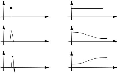
In communication systems, real impulsive-type noise has a duration that is normally more than one sample long. For example, in the context of audio signals, short-duration, sharp pulses, of up to 3 milliseconds (60 samples at a 20 kHz sampling rate) may be considered as impulsive-type noise. Figures 12.1(b) and 12.1(c) illustrate two examples of short-duration pulses and their respective spectra.

Figure 12.2 Time and frequency sketches of (a) an ideal impulse, and (b) and (c) short-duration pulses.

Figure 12.3 Illustration of variations of the impulse response of a non-linear system with increasing amplitude of the impulse.

In a communication system, an impulsive noise originates at some point in time and space, and then propagates through the channel to the receiver. The received noise is shaped by the channel, and can be considered as the channel impulse response. In general, the characteristics of a communication channel may be linear or non-linear, stationary or time varying. Furthermore, many communication systems, in response to a large-amplitude impulse, exhibit a nonlinear characteristic.

Figure 12.3 illustrates some examples of impulsive noise, typical of those observed on an old gramophone recording. In this case, the communication channel is the playback system, and may be assumed timeinvariant. The figure also shows some variations of the channel characteristics with the amplitude of impulsive noise. These variations may be attributed to the non-linear characteristics of the playback mechanism.

An important consideration in the development of a noise processing system is the choice of an appropriate domain (time or the frequency) for signal representation. The choice should depend on the specific objective of the system. In signal restoration, the objective is to separate the noise from the signal, and the representation domain must be the one that emphasises the distinguishing features of the signal and the noise. Impulsive noise is normally more distinct and detectable in the time domain than in the frequency domain, and it is appropriate to use timedomain signal processing for noise detection and removal. In signal classification and parameter estimation, the objective may be to compensate for the average effects of the noise over a number of samples, and in some cases, it may be more appropriate to process the impulsive noise in the frequency domain where the effect of noise is a change in the mean of the power spectrum of the signal.

12.1.1 Autocorrelation and Power Spectrum of Impulsive Noise

Impulsive noise is a non-stationary, binary-state sequence of impulses with random amplitudes and random positions of occurrence. The non-stationary nature of impulsive noise can be seen by considering the power spectrum of a noise process with a few impulses per second: when the noise is absent the process has zero power, and when an impulse is present the noise power is the power of the impulse. Therefore the power spectrum and hence the autocorrelation of an impulsive noise is a binary state, time-varying process. An impulsive noise sequence can be modelled as an amplitude-modulated binary-state sequence, and expressed as

where b(m) is a binary-state random sequence of ones and zeros, and n(m) is a random noise process. Assuming that impulsive noise is an uncorrelated random process, the autocorrelation of impulsive noise may be defined as a binary-state process:

where δ(k) is the Kronecker delta function. Since it is assumed that the noise is an uncorrelated process, the autocorrelation is zero for k ≠ 0 , therefore Equation (12.7) may be written as

Note that for a zero-mean noise process, rnn(0,m) is the time-varying binary-state noise power. The power spectrum of an impulsive noise sequence is obtained, by taking the Fourier transform of the autocorrelation function Equation (12.8), as

In Equation (12.8) and (12.9) the autocorrelation and power spectrum are expressed as binary state functions that depend on the “on/off” state of impulsive noise at time m.

process n(m). A Bernoulli process b(m) is a binary-valued process that takes a value of “1” with a probability of α and a value of “0” with a probability of 1–α. Τhe probability mass function of a Bernoulli process is given by

and a variance

A zero-mean Gaussian pdf model of the random amplitudes of impulsive noise is given by

where σn2 is the variance of the noise amplitude. In a Bernoulli–Gaussian model the probability density function of an impulsive noise ni(m) is given by

where δ (ni (m)) is the Kronecker delta function. Note that the function is a mixture of a discrete probability mass function δ (ni (m))

and a continuous probability density function f N (ni (m)).

An alternative model for impulsive noise is a binary-state Gaussian process (Section 2.5.4), with a low-variance state modelling the absence of impulses and a relatively high-variance state modelling the amplitude of impulsive noise.

12.2.2 Poisson–Gaussian Model of Impulsive Noise

In a Poisson–Gaussian model the probability of occurrence of an impulsive noise event is modelled by a Poisson process, and the distribution of the random amplitude of impulsive noise is modelled by a Gaussian process. The Poisson process, described in Chapter 2, is a random event-counting process. In a Poisson model, the probability of occurrence of k impulsive noise in a time interval of T is given by

k!

where λ is a rate function with the following properties:

Prob(one impulse in a small time interval û9 )= λû9

( ) (12.17) Prob zero impulse in a small time interval û9 =1−λû9

It is assumed that no more than one impulsive noise can occur in a time interval ∆t. In a Poisson–Gaussian model, the pdf of an impulsive noise ni(m) in a small time interval of ∆t is given by

where f N (ni (m)) is the Gaussian pdf of Equation (12.14).

12.2.3 A Binary-State Model of Impulsive Noise

An impulsive noise process may be modelled by a binary-state model as shown in Figure 12.4. In this binary model, the state S0 corresponds to the “off” condition when impulsive noise is absent; in this state, the model emits zero-valued samples. The state S1 corresponds to the “on” condition; in this state the model emits short-duration pulses of random amplitude and duration. The probability of a transition from state Si to state Sj is denoted by aij. In its simplest form, as shown in Figure 12.5, the model is memoryless, and the probability of a transition to state Si is independent of the current state of the model. In this case, the probability that at time t+1

a =1 - α

00

a =1 - α

10

Figure 12.5 A binary-state model of an impulsive noise generator.

Figure 12.6 A 3-state model of impulsive noise and the decaying oscillations that often follow the impulses.

the signal is in the state S0 is independent of the state at time t, and is given by

P(s(t +1) = S0 s(t) = S0 ) = P(s(t +1) = S0 s(t) = S1 )=1− α (12.19)

where st denotes the state at time t. Likewise, the probability that at time t+1 the model is in state S1 is given by

In a more general form of the binary-state model, a Markovian statetransition can model the dependencies in the noise process. The model then becomes a 2-state hidden Markov model considered in Chapter 5.

In one of its simplest forms, the state S1 emits samples from a zero-mean Gaussian random process. The impulsive noise model in state S1 can be configured to accommodate a variety of impulsive noise of different shapes,

durations and pdfs. A practical method for modelling a variety of impulsive noise is to use a code book of M prototype impulsive noises, and their associated probabilities [(ni1, pi1), (ni2 , pi2), ..., (niM , piM)], where pj denotes the probability of impulsive noise of the type nj. The impulsive noise code book may be designed by classification of a large number of “training” impulsive noises into a relatively small number of clusters. For each cluster, the average impulsive noise is chosen as the representative of the cluster. The number of impulses in the cluster of type j divided by the total number of impulses in all clusters gives pj, the probability of an impulse of type j.

Figure 12.6 shows a three-state model of the impulsive noise and the decaying oscillations that might follow the noise. In this model, the state S0 models the absence of impulsive noise, the state S1 models the impulsive noise and the state S2 models any oscillations that may follow a noise pulse.

12.2.4 Signal to Impulsive Noise Ratio

For impulsive noise the average signal to impulsive noise ratio, averaged over an entire noise sequence including the time instances when the impulses are absent, depends on two parameters: (a) the average power of each impulsive noise, and (b) the rate of occurrence of impulsive noise. Let Pimpulse denote the average power of each impulse, and Psignal the signal power. We may define a “local” time-varying signal to impulsive noise ratio as

The average signal to impulsive noise ratio, assuming that the parameter α is the fraction of signal samples contaminated by impulsive noise, can be defined as

Note that from Equation (12.22), for a given signal power, there are many pair of values of α and PImpulse that can yield the same average SINR.