Добавил:

korayakov Опубликованный материал нарушает ваши авторские права? Сообщите нам.

Вуз:

Национальный исследовательский университет «МИЭТ»

Предмет:

Цифровая обработка сигналов

Файл:

10 - Interpolation

.pdf

Скачиваний:

Добавлен:

17.04.2013

Размер:

288 Кб

Скачать

☆

<<< < Предыдущая 1 23 / 43 4 > Следующая >>>

Model-Based Interpolation

317

10.3.3 Interpolation Based on a Short-Term Prediction Model

An autoregressive (AR), or linear predictive, signal x(m) is described as

P
x(m) =∑ak x(m − k)+e(m)	(10.53)

k =1

where x(m) is the AR signal, ak are the model coefficients and e(m) is a zero mean excitation signal. The excitation may be a random signal, a quasiperiodic impulse train, or a mixture of the two. The AR coefficients, ak, model the correlation structure or equivalently the spectral patterns of the signal.

Assume that we have a signal record of N samples and that within this record a segment of M samples, starting from the sample k, xUk={x(k), ...,

x(k+M–1)} are missing. The objective is to estimate the missing samples xUk, using the remaining N–k samples and an AR model of the signal.

Figure 10.8 illustrates the interpolation problem. For this signal record of N samples, the AR equation (10.53) can be expanded to form the following matrix equation:

	e(P )		x( P)		x( P − 1)
	e( P + 1)		x( P + 1)		x( P)
	e( P + 1)		x( P + 1)		x( P)



	e(k − 1)		x(k − 1)		x(k − 2)
	e(k )		xUk ( k )		x(k − 1)
	e(k )		xUk ( k )		x(k − 1)
	e(k + 1)		xUk ( k + 1 )		xUk ( k )
	e(k + 2)		xUk ( k + 2 )		xUk ( k + 1 )
	e(k + 2)	=	xUk ( k + 2 )	−	xUk ( k + 1 )


e(k + M + P − 2)		x(k + M + P − 2)		x(k + M + P − 3)
e(k + M + P − 1)			x(k + M + P − 1)	x(k + M + P − 2)

e(k + M + P)		x(k + M + P )		x(k + M + P − 1)
					x(k + M + P )
e(k + M + P + 1)		x(k + M + P + 1)			x(k + M + P )

	e( N − 1)		x( N − 1)		x( N − 2)
	e( N − 1)		x( N − 1)		x( N − 2)

x( P − 2) x( P − 1)

x(k − 3) x(k − 2) x(k − 1)

xUk ( k )

x(k + M + P − 2) x(k + M + P − 1) x(k + M + P )

x(k + M + P + 1)

x( N − 3)

		x(0)
		x(1)
		x(1)



	x(k − P − 1)
	x(k − P)
	x(k − P)			a
	x(k − P + 1)			a
	x(k − P + 1)				1
	x(k − P + 2)			a2
	x(k − P + 2)			a
				a
					3

xUk ( k + M − 2 )
x	Uk	( k + M −	1 )	aP
	Uk
	x(k + M )
	x(k + M + 1)
	x(k + M + 1)

	x( N − P − 1)
	x( N − P − 1)

(10.54)

where the subscript Uk denotes the unknown samples. Equation (10.54) can be rewritten in compact vector notation as

318	Interpolation
e( x Uk ,a )= x−Xa	(10.55)

where the error vector e(xUk, a) is expressed as a function of the unknown samples and the unknown model coefficient vector. In this section, the optimality criteriobbn for the estimation of the model coefficient vector a and the missing samples xUk is the minimum mean square error given by the inner vector product

e T e( x Uk , a )= x T x+a T X T Xa − 2a T X T x

(10.56)

The squared error function in Equation (10.56) involves nonlinear unknown terms of fourth order, aTXTXa, and cubic order, aTXTx. The least square error formulation, obtained by differentiating eTe(xUk ,a), with respect to the vectors a or xUk, results in a set of nonlinear equations of cubic order whose solution is non-trivial. A suboptimal, but practical and mathematically tractable, approach is to solve for the missing samples and the unknown model coefficients in two separate stages. This is an instance of the general estimate-and-maximise (EM) algorithm, and is similar to the linearpredictive model-based restoration considered in Section 6.7. In the first stage of the solution, Equation (10.54) is linearised by either assuming that the missing samples have zero values or discarding the set of equations in (10.54), between the two dashed lines, that involve the unknown signal samples. The linearised equations are used to solve for the AR model coefficient vector a by forming the equation

ˆ ( T	)−1( T	)	(10.57)
a = X Kn X Kn	X Kn xKn		(10.57)

where the vector is an estimate of the model coefficients, obtained from the available signal samples.

The second stage of the solution involves the estimation of the unknown signal samples xUk. For an AR model of order P, and an unknown

signal segment of length M, there are 2M+P nonlinear equations in (10.54) that involve the unknown samples; these are

Model-Based Interpolation

319

	e(k )			x	Uk	(k )
					Uk
	e(k + 1)			xUk (k + 1)
	e(k + 2)	=		xUk (k + 2)			−
	e(k + 2)			xUk (k + 2)


e(k + M + P − 2)			x(k + M + P − 2)					xUk

e(k + M + P − 1)			x(k + M + P − 1)					xUk

x(k − 1)

xUk (k )

xUk (k + 1)

(k + M + P − 3)

(k + M + P − 2)

x(k − 2)

x(k − 1)

xUk (k )

xUk (k + M + P − 4) xUk (k + M + P − 3)

x(k − p)		a1

x(k − p + 1)		a2
x(k − p + 2)			a
			3

xUk (k + M −
xUk (k + M −	2)	aP-1
xUk (k + M −
xUk (k + M −	1) aP

(10.58)

The estimate of the predictor coefficient vector , obtained from the first stage of the solution, is substituted in Equation (10.58) so that the only remaining unknowns in (10.58) are the missing signal samples. Equation (10.58) may be partitioned and rearranged in vector notation in the following form:

	e(k)
	e(k +1)
	e(k +1)
	e(k + 2)
	e(k + 2)
	e(k + 3)
	e(k + 4)

			=
	e(k + P −1)		=
	e(k + P)
	e(k + P)
	e(k + P +1)
	e(k + P +1)
		− 2)
e(k + M + P		− 2)

e(k + M + P −1)

	1
	− a
	1
	− a2
	− a3
	− a4

	− aP
	0
	0
	0

	0
	0
	0

0	0	0
1	0	0
− a1	1	0
− a2	− a1	1
− a3	− a2	− a1

− aP−1	− aP −2	− aP−3
− aP	− aP−1	− aP−2
0	− aP	− aP−1

0	0	0
0	0	0

	0
	0
	0		xUk (k )
	0		xUk (k )
	0
	0		xUk (k + 1)
	0		xUk (k + 1)
	0
			xUk (k + 2)		+
			xUk (k + 2)		+
0			xUk (k + 3)
0			xUk (k + 3)
	0
	0
	0

xUk (k + M −				1)
	− a	P−1
		P−1
	− aP

	− a	P	− a	P−1	− a	P−2		− a	0	0		0	0
								1
	0		− aP		− aP−1		− a2		0	0		0	0
0			0		− aP		− a3		0	0		0	0

0			0		0			− aP	0	0		0	0
	0		0		0		0		0	0		0	0
	0		0		0		0		0		1	0	0
	0		0		0		0		0		− a	1	0
	0		0		0		0		0		− a1	− a	1
											2	1	− a1
0			0		0		0		0	− a3		− a2

			0		0		0		0	− aP−1		− aP−2	− aP−3
0

−

	x(k − P)
	x(k − P + 1)
	x(k − P + 1)
	x(k − P + 2)

	x(k − 1)
	x(k − 1)
	0

	x(k + M )
	x(k + M + 1)
	x(k + M + 2)


	x(k + M + P −
	x(k + M + P −	1)

(10.59) In Equation (10.59), the unknown and known samples are rearranged and grouped into two separate vectors. In a compact vector–matrix notation, Equation (10.58) can be written in the form

e= A1 xUk + A2 xKn

(10.60)

320 Interpolation

where e is the error vector, A1 is the first coefficient matrix, xUk is the unknown signal vector being estimated, A2 is the second coefficient matrix and the vector xKn consists of the known samples in the signal matrix and vectors of Equation (10.58). The total squared error is given by

eT e= (A x	Uk	+ A x	Kn	)T (A x	Uk	+ A x	Kn	)	(10.61)
1	Uk	2	Kn	1	Uk	2	Kn

The least square AR (LSAR) interpolation is obtained by minimisation of the squared error function with respect to the unknown signal samples xUk:

∂

=2AT A x

+2AT A x

= 0

(10.62)

∂ xUk

From Equation (10.62) we have

ˆ LSAR

(

)−1( T

)

(10.63)

xUk

=− A1

xKn

ˆ LSAR

The solution in Equation (10.62) gives the

xUk , vector which is the least

square error estimate of the unknown data vector.

10.3.4 Interpolation Based on Long-Term and Short-term Correlations

For the best results, a model-based interpolation algorithm should utilise all the correlation structures of the signal process, including any periodic structures. For example, the main correlation structures in a voiced speech signal are the short-term correlation due to the resonance of the vocal tract and the long-term correlation due to the quasi-periodic excitation pulses of the glottal cords. For voiced speech, interpolation based on the short-term correlation does not perform well if the missing samples coincide with an underlying quasi-periodic excitation pulse. In this section, the AR interpolation is extended to include both long-term and short-term correlations. For most audio signals, the short-term correlation of each sample with the immediately preceding samples decays exponentially with time, and can be usually modelled with an AR model of order 10–20. In order to include the pitch periodicities in the AR model of Equation (10.53),

Model-Based Interpolation

321

2Q+1 samples a	P past samples
pitch period away

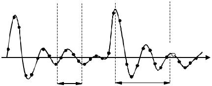
Figure 10.10 A quasiperiodic waveform. The sample marked “ ? ” is predicted using P immediate past samples and 2Q+1 samples a pitch period away.

the model order must be greater than the pitch period. For speech signals, the pitch period is normally in the range 4–20 milliseconds, equivalent to 40–200 samples at a sampling rate of 10 kHz. Implementation of an AR model of this order is not practical owing to stability problems and computational complexity.

A more practical AR model that includes the effects of the long-term correlations is illustrated in Figure 10.10. This modified AR model may be expressed by the following equation:

P	Q
x(m) = ∑ak x(m − k) +	∑ pk x(m − T − k) + e(m)	(10.64)
k=1	k =−Q

The AR model of Equation (10.64) is composed of a short-term predictor Σak x(m-k) that models the contribution of the P immediate past samples, and a long-term predictor Σpk x(m–T–k) that models the contribution of 2Q+1 samples a pitch period away. The parameter T is the pitch period; it can be estimated from the autocorrelation function of x(m) as the time difference between the peak of the autocorrelation, which is at the correlation lag zero, and the second largest peak, which should happen a pitch period away from the lag zero.

The AR model of Equation (10.64) is specified by the parameter vector c=[a1, ..., aP, p–Q, ..., pQ] and the pitch period T. Note that in Figure 10.10

322		Interpolation
xKn1	xUk	xKn2

? ... ?

		M missing
2Q+1	P samples	samples
2Q+1	P samples	P samples	2Q+1
samples	before	after	samples

Figure 10.11 A signal with M missing samples. P immediate samples each side of the gap and 2Q+1 samples a pitch period away are used for interpolation.

the sample marked “?” coincides with the onset of an excitation pulse. This sample is not well predictable from the P past samples, because they do not include a pulse event. The sample is more predictable from the 2Q+1 samples a pitch period away, since they include the effects of a similar excitation pulse. The predictor coefficients are estimated (see Chapter 7) using the so-called normal equations:

c = Rxx−1 rxx

(10.65)

where Rxx is the autocorrelation matrix of signal x and rxx is the correlation vector. In expanded form, Equation (10.65) can be written as

a1				r(0)	r(1)	r(P − 1)
	a2			r(1)	r(0)		r(P − 2)
	a2			r(1)	r(0)		r(P − 2)
	a3			r(2)	r(1)	r(P − 3)


	aP	=		r(P − 1)	r(P − 2)		r(0)
	aP	=		r(P − 1)	r(P − 2)		r(0)
	p−Q		r(T + Q − 1) r(T + Q − 2)			r(T + Q − P)
				r(T + Q)	r(T + Q − 1)	r(T + Q − P + 1)
p−Q+1				r(T + Q)	r(T + Q − 1)	r(T + Q − P + 1)


	p+Q		r(T − Q − 1) r(T − Q − 2) r(T − Q − P)
	p+Q		r(T − Q − 1) r(T − Q − 2) r(T − Q − P)

r(T + Q − 1)	r(T + Q)
r(T + Q − 2)	r(T + Q − 1)
r(T + Q − 3)	r(T + Q − 2)

r(T + Q − P) r(T + Q − P + 1)

r(0)	r(1)
r(1)	r(0)

r(2Q)

r(2Q − 1)

r(T − Q − 1) −1				r(1)

	r(T + Q −	2)		r(2)

	r(T + Q −	3)		r(3)


	r(T + Q −	P)		r(P)
	r(2Q)			r(T + Q)

	r(2Q − 1)		r(T + Q − 1)

	r(0)
	r(0)			r(T − Q)

(10.66) The modified AR model can be used for interpolation in the same way as the conventional AR model described in the previous section. Again, it is assumed that within a data window of N speech samples, a segment of M samples commencing from the sample point k, xUk={x(k), x(k+1), ...,

Model-Based Interpolation

323

x(k+M–1)} is missing. Figure 10.11 illustrates the interpolation problem. The missing samples are estimated using P samples in the immediate vicinity and 2Q+1 samples a pitch period away on each side of the missing signal. For the signal record of N samples, the modified AR equation (10.64) can be written in matrix form as

	e(T	+ Q)			x(T + Q)		x(T + Q − 1)
								x(T + Q)
e(T + Q + 1)				x(T + Q + 1)				x(T + Q)



	e(k	− 1)			x(k − 1)			x(k − 2)
	e(k )				xUK (k)			x(k − 1)
	e(k )				xUK (k)			x(k − 1)
	e(k	+ 1)			xUK (k + 1)			xUK (k)
	e(k	+ 1)			xUK (k + 1)			xUK (k)
	e(k		=		xUK (k + 2)	−		xUK (k + 1)
	e(k	+ 2)			xUK (k + 2)			xUK (k + 1)



e(k + M + P − 2)				x(k + M + P − 2)			x(k + M + P − 3)

e(k + M		+ P − 1)		x(k + M + P − 1)			x(k + M + P − 2)
e(k + M + P)				x(k + M + P)			x(k + M + P − 1)
								x(k + M + P)
e(k + M		+ P + 1)		x(k + M + P + 1)				x(k + M + P)


	e(N	− 1)			x(N − 1)			x(N − 2)
	e(N	− 1)			x(N − 1)			x(N − 2)

x(T + Q − P)

x(T + Q − P + 1)

x(k − P − 1)

x(k − P)

x(k − P + 1)

x(k − P + 2)

xUK (k + M − 2)

xUK (k + M − 1)

x(k + M )

x(k + M + 1)

x(N − P − 1)

x(2Q) x(2Q + 1)

x(k − T + Q − 1) x(k − T + Q) x(k − T + Q + 1) x(k − T + Q + 2)

x(k + M + P − T + Q − 2) x(k + M + P − T + Q − 1) x(k + M + P − T + Q) x(k + M + P − T + Q + 1)

x(N − T + Q − 1)

x(0)

x(1)



x(k − T − Q − 1)			a
			1
x(k − T − Q)		a2

x(k − T − Q + 1)			a3


x(k − T − Q + 2)


			aP

x(k + M + P − T − Q −		p
	2)
			−Q
x(k + M + P − T − Q −	1)

x(k + M + P − T − Q)
		p+Q
x(k + M + P − T − Q +
	1)


x(N − T − Q − 1)

(10.67) where the subscript Uk denotes the unknown samples. In compact matrix notation, this set of equation can be written in the form

e( xUk ,c )= x+ Xc

(10.68)

As in Section 10.3.2, the interpolation problem is solved in two stages:

(a)In the first stage, the known samples on both sides of the missing signal are used to estimate the AR coefficient vector c.

(b)In the second stage, the AR coefficient estimates are substituted in Equation (10.68) so that the only unknowns are the data samples.

The solution follows the same steps as those described in Section 10.3.2.

10.3.5 LSAR Interpolation Error

In this section, we discuss the effects of the signal characteristics, the model parameters and the number of unknown samples on the interpolation error. The interpolation error v(m), defined as the difference between the original sample x(m) and the interpolated sample xˆ(m) , is given by

324	Interpolation
v(m) = x(m) − xˆ(m)	(10.69)

A common measure of signal distortion is the mean square error distance defined as

D(c,M )	=	1	M −1[	+	m)	− ˆ	+	m)	]2
										(10.70)
		M	E ∑ x(k			x(k
			m=0

where k is the beginning of an M-samples long segment of missing signal, and E [.] is the expectation operator. In Equation (10.70), the average distortion D is expressed as a function of the number of the unknown samples M, and also the model coefficient vector c. In general, the quality of interpolation depends on the following factors:

(a)The signal correlation structure. For deterministic signals such as sine waves, the theoretical interpolation error is zero. However information-bearing signals have a degree of randomness that makes perfect interpolation with zero error an impossible objective.

(b)The length of the missing segment. The amount of information lost, and hence the interpolation error, increase with the number of missing samples. Within a sequence of missing samples the error is usually largest for the samples in the middle of the gap. The interpolation Equation (10.63) becomes increasingly ill-conditioned as the length of the missing samples increases.

(c)The nature of the excitation underlying the missing samples. The LSAR interpolation cannot account for any random excitation underlying the missing samples. In particular, the interpolation quality suffers when the missing samples coincide with the onset of an excitation pulse. In general, the least square error criterion causes the interpolator to underestimate the energy of the underlying excitation signal. The inclusion of long-term prediction and the use of quasi-periodic structure of signals improves the ability of the interpolator to restore the missing samples.

(d)AR model order and the method used for estimation of the AR coefficients. The interpolation error depends on the AR model order. Usually a model order of 2–3 times the length of missing data sequence achieves good result.

Model-Based Interpolation

325

2500									1000
2000
1500									500
1000
500									0
0
-500									-500
-500
-1000
-1500									-1000
-1500
-2000
-2500									-1500
-2500	50	100	150	200	250	300	350	400	0
0	50	100	150	200	250	300	350	400
				(a)
2500									1000
2500
2000
1500									500
1500
1000
500									0
500
0
-500									-500
-500
-1000
-1500									-1000
-1500
-2000
-2500	50	100	150	200	250	300	350	400	-1500
0	50	100	150	200	250	300	350	400	0
				(b)

100

150

200

250

300

350

400

(a)

100

150

200

250

300

350

400

(b)

Figure 10.12 (a) A section of speech	Figure 10.13	(a) A section of speech
showing interpolation of 60 samples	showing interpolation of 50 samples
starting from the sample point 100 (b)	starting from the sample point 175 (b)
Interpolation using short and long-term	Interpolation using short and long-term
correlations. Interpolated samples are	correlations.	Interpolated samples are
shown by the light shaded line.	shown by the light shaded line.

The interpolation error also depends on how well the AR parameters can be estimated from the incomplete data. In Equation (10.54), in the first stage of the solution, where the AR coefficients are estimated, two different approaches may be employed to linearise the system of equations. In the first approach all equations, between the dashed lines, that involve nonlinear terms are discarded. This approach has the advantage that no assumption is made about the missing samples. In fact, from a signalensemble point of view, the effect of discarding some equations is

326	Interpolation

equivalent to that of having a smaller signal record. In the second method, starting from an initial estimate of the unknown vector (such as xUk=0), Equation (10.54) is solved to obtain the AR parameters. The AR coefficients are then used in the second stage of the algorithm to estimate the unknown samples. These estimates may be improved in further iterations of the algorithm. The algorithm usually converges after one or two iterations.

Figures 10.12 and 10.13 show the results of application of the least square error AR interpolation method to speech signals. The interpolated speech segments were chosen to coincide with the onset of an excitation pulse. In these experimental cases the original signals are available for comparison. Each signal was interpolated by the AR model of Equation (10.53) and also by the extended AR model of Equation (10.64). The length of the conventional linear predictor model was set to 20. The modified linear AR model of Equation (10.64) has a prediction order of (20,7); that is, the short-term predictor has 20 coefficients and the long-term predictor has 7 coefficients. The figures clearly demonstrate that the modified AR model that includes the long-term as well as the short-term correlation structures outperforms the conventional AR model.

10.3.6 Interpolation in Frequency–Time Domain

Time-domain, AR model-based interpolation methods are effective for the interpolation of a relatively short length of samples (say less than 100 samples at a 20 kHz sampling rate), but suffer severe performance degradations when used for interpolation of large sequence of samples. This is partly due to the numerical problems associated with the inversion of a large matrix, involved in the time-domain interpolation of a large number of samples, Equation (10.58).

Spectral–time representation provides a useful form for the interpolation of a large gap of missing samples. For example, through discrete Fourier transformation (DFT) and spectral–time representation of a signal, the problem of interpolation of a gap of N samples in the time domain can be converted into the problem of interpolation of a gap of one sample, along the time, in each of N discrete frequency bins, as explained next.

Spectral–Time Representation with STFT

A relatively simple and practical method for spectral–time representation of a signal is the short-time Fourier transform (STFT) method. To construct a

<<< < Предыдущая 1 23 / 43 4 > Следующая >>>

Соседние файлы в папке Advanced Digital Signal Processing and Noise Reduction (Saeed V. Vaseghi)

#
17.04.2013258.04 Кб3305 - Hidden Markov models.pdf
#
17.04.2013202.47 Кб3606 - Wiener filters.pdf
#
17.04.2013142.76 Кб3607 - Adaptive filters.pdf
#
17.04.2013260.56 Кб3208 - Linear prediction models.pdf
#
17.04.2013237.7 Кб3309 - Power spectrum and correlation.pdf
#
17.04.2013288 Кб3210 - Interpolation.pdf
#
17.04.2013363.44 Кб3411 - Spectral subtraction.pdf
#
17.04.2013188.5 Кб3312 - Impulsive noise.pdf
#
17.04.2013484.69 Кб3213 - Transient noise pulses.pdf
#
17.04.2013141.02 Кб3514 - Echo cancellation.pdf
#
17.04.2013331.48 Кб3615 - Channel equalization and blind deconvolution.pdf