electrodynamics / Electromagnetic Field Theory - Bo Thide

purpose of the limiting process is to assure that the test charge q does not influence the field, the expression for Estat does not depend explicitly on q but only on the charge q0 and the relative radius vector x x0. This means that we can say that any net electric charge produces an electric field in the space that surrounds it, regardless of the existence of a second charge anywhere in this space.1

Using formulae (1.1) and (1.2), we find that the electrostatic field Estat at the field point x (also known as the observation point), due to a field-producing charge q0 at the source point x0, is given by

In the presence of several field producing discrete charges q0i , at x0i , i =1;2;3;:::, respectively, the assumption of linearity of vacuum2 allows us to superimpose their individual E fields into a total E field

If the discrete charges are small and numerous enough, we introduce the charge density located at x0 and write the total field as

where, in the last step, we used formula Equation (M.68) on page 172. We emphasise that Equation (1.5) above is valid for an arbitrary distribution of charges, including discrete charges, in which case can be expressed in terms of one or more Dirac delta functions.

1In the preface to the first edition of the first volume of his book A Treatise on Electricity and Magnetism, first published in 1873, James Clerk Maxwell describes this in the following, almost poetic, manner: [6]

“For instance, Faraday, in his mind's eye, saw lines of force traversing all space where the mathematicians saw centres of force attracting at a distance: Faraday saw a medium where they saw nothing but distance: Faraday sought the seat of the phenomena in real actions going on in the medium, they were satisfied that they had found it in a power of action at a distance impressed on the electric fluids.”

2In fact, vacuum exhibits a quantum mechanical nonlinearity due to vacuum polarisation effects manifesting themselves in the momentary creation and annihilation of electron-positron pairs, but classically this nonlinearity is negligible.

Since, according to formula Equation (M.78) on page 175, r [r (x)] 0 for any 3D 3 scalar field (x), we immediately find that in electrostatics

I.e., Estat is an irrotational field.

Taking the divergence of the general Estat expression for an arbitrary charge distribution, Equation (1.5) on the preceding page, and using the representation

which is Gauss's law in differential form.

1.2 Magnetostatics

While electrostatics deals with static charges, magnetostatics deals with stationary currents, i.e., charges moving with constant speeds, and the interaction between these currents.

1.2.1 Ampère's law

Experiments on the interaction between two small current loops have shown that they interact via a mechanical force, much the same way that charges interact. Let F denote such a force acting on a small loop C carrying a current J located at x, due to the presence of a small loop C0 carrying a current J0

J

C dl

x

C0

J0

x0

O

FIGURE 1.2: Ampère's law describes how a small loop C, carrying a static electric current J through its tangential line element dl located at x, experiences a magnetostatic force from a small loop C0, carrying a static electric current J0 through the tangential line element dl0 located at x0. The loops can have arbitrary shapes as long as they are simple and

closed.

located at x0. According to Ampère's law this force is, in vacuum, given by the expression

Here dl and dl0 are tangential line elements of the loops C and C0, respectively, and, in SI units, 0 = 4 10 7 1:2566 10 6 H/m is the vacuum permeability. From the definition of "0 and 0 (in SI units) we observe that

which is a useful relation.

At first glance, Equation (1.8) above appears to be unsymmetric in terms of the loops and therefore to be a force law which is in contradiction with Newton's third law. However, by applying the vector triple product “bac-cab”

formula (F.54) on page 155, we can rewrite (1.8) in the following way

Recognising the fact that the integrand in the first integral is an exact differential so that this integral vanishes, we can rewrite the force expression, Equation (1.8) on the previous page, in the following symmetric way

This clearly exhibits the expected symmetry in terms of loops C and C0.

1.2.2 The magnetostatic field

In analogy with the electrostatic case, we may attribute the magnetostatic interaction to a vectorial magnetic field Bstat. I turns out that Bstat can be defined through

which expresses the small element dBstat(x) of the static magnetic field set up at the field point x by a small line element dl0 of stationary current J0 at the source point x0. The SI unit for the magnetic field, sometimes called the magnetic flux density or magnetic induction, is Tesla (T).

If we generalise expression (1.12) to an integrated steady state current distribution j(x), we obtain Biot-Savart's law:

= 4 V j(x0) r jx x0j d3x0

Comparing Equation (1.5) on page 3 with Equation (1.13), we see that there exists a close analogy between the expressions for Estat and Bstat but that they differ in their vectorial characteristics. With this definition of Bstat, Equation (1.8) on the previous page may we written

F(x) = J dl Bstat(x) (1.14)

C

In order to assess the properties of Bstat, we determine its divergence and curl. Taking the divergence of both sides of Equation (1.13) on the facing page and utilising formula (F.61) on page 155, we obtain

where the first term vanishes because j(x0) is independent of x so that r j(x0) 0, and the second term vanishes since, according to Equation (M.78) on page 175, r [r (x)] vanishes for any scalar field (x).

Applying the operator “bac-cab” rule, formula (F.67) on page 155, the curl

In the first of the two integrals on the right hand side, we use the representation of the Dirac delta function Equation (M.73) on page 174, and integrate the second one by parts, by utilising formula (F.59) on page 155 as follows:

Then we note that the first integral in the result, obtained by applying Gauss's theorem, vanishes when integrated over a large sphere far away from the localised source j(x0), and that the second integral vanishes because r j = 0 for

stationary currents (no charge accumulation in space). The net result is simply

1.3 Electrodynamics

As we saw in the previous sections, the laws of electrostatics and magnetostatics can be summarised in two pairs of time-independent, uncoupled vector differential equations, namely the equations of classical electrostatics3

Since there is nothing a priori which connects Estat directly with Bstat, we must consider classical electrostatics and classical magnetostatics as two independent theories.

However, when we include time-dependence, these theories are unified into one theory, classical electrodynamics. This unification of the theories of electricity and magnetism is motivated by two empirically established facts:

1.Electric charge is a conserved quantity and current is a transport of electric charge. This fact manifests itself in the equation of continuity and, as a consequence, in Maxwell's displacement current.

2.A change in the magnetic flux through a loop will induce an EMF electric field in the loop. This is the celebrated Faraday's law of induction.

3The famous physicist and philosopher Pierre Duhem (1861–1916) once wrote:

“The whole theory of electrostatics constitutes a group of abstract ideas and general propositions, formulated in the clear and concise language of geometry and algebra, and connected with one another by the rules of strict logic. This whole fully satisfies the reason of a French physicist and his taste for clarity, simplicity and order. . . ”

1.3.1 Equation of continuity

Let j denote the electric current density (A/m2). In the simplest case it can be defined as j =v where v is the velocity of the charge density. In general, j has to be defined in statistical mechanical terms as j(t;x) = å q v f (t;x;v)d3v where f (t;x;v) is the (normalised) distribution function for particle species with electrical charge q .

The electric charge conservation law can be formulated in the equation of continuity

which states that the time rate of change of electric charge (t;x) is balanced by a divergence in the electric current density j(t;x).

1.3.2 Maxwell's displacement current

We recall from the derivation of Equation (1.18) on the preceding page that there we used the fact that in magnetostatics r j(x) = 0. In the case of nonstationary sources and fields, we must, in accordance with the continuity Equation (1.21), set r j(t;x) = @ (t;x)=@t. Doing so, and formally repeating the steps in the derivation of Equation (1.18) on the preceding page, we would obtain the formal result

where, in the last step, we have assumed that a generalisation of Equation (1.5) on page 3 to time-varying fields allows us to make the identification

Later, we will need to consider this formal result further. The result is Maxwell's source equation for the B field

where the last term @"0E(t;x)=@t is the famous displacement current. This term was introduced, in a stroke of genius, by Maxwell in order to make the right hand side of this equation divergence free when j(t;x) is assumed to represent the density of the total electric current, which can be split up in “ordinary” conduction currents, polarisation currents and magnetisation currents. The displacement current is an extra term which behaves like a current density flowing in vacuum. As we shall see later, its existence has far-reaching physical consequences as it predicts the existence of electromagnetic radiation that can carry energy and momentum over very long distances, even in vacuum.

1.3.3 Electromotive force

If an electric field E(t;x) is applied to a conducting medium, a current density j(t;x) will be produced in this medium. There exist also hydrodynamical and chemical processes which can create currents. Under certain physical conditions, and for certain materials, one can sometimes assume a linear relationship between the current density j and E, called Ohm's law:

where is the electric conductivity (S/m). In the most general cases, for instance in an anisotropic conductor, is a tensor.

We can view Ohm's law, Equation (1.25) above, as the first term in a Taylor expansion of the law j[E(t;x)]. This general law incorporates non-linear effects such as frequency mixing. Examples of media which are highly non-linear are semiconductors and plasma. We draw the attention to the fact that even in cases when the linear relation between E and j is a good approximation, we still have to use Ohm's law with care. The conductivity is, in general, time-dependent (temporal dispersive media) but then it is often the case that Equation (1.25) is valid for each individual Fourier component of the field.

If the current is caused by an applied electric field E(t;x), this electric field will exert work on the charges in the medium and, unless the medium is superconducting, there will be some energy loss. The rate at which this energy is expended is j E per unit volume. If E is irrotational (conservative), j will decay away with time. Stationary currents therefore require that an electric field which corresponds to an electromotive force (EMF) is present. In the presence of such a field EEMF, Ohm's law, Equation (1.25) above, takes the form

where dl is a tangential line element of the closed loop C.

1.3.4 Faraday's law of induction

In Subsection 1.1.2 we derived the differential equations for the electrostatic field. In particular, on page 4 we derived Equation (1.6) which states that r Estat(x) = 0 and thus that Estat is a conservative field (it can be expressed as a gradient of a scalar field). This implies that the closed line integral of Estat in Equation (1.27) above vanishes and that this equation becomes

E = EEMF dl (1.28)

C

It has been established experimentally that a nonconservative EMF field is produced in a closed circuit C if the magnetic flux through this circuit varies with time. This is formulated in Faraday's law which, in Maxwell's generalised form, reads

where m is the magnetic flux and S is the surface encircled by C which can be interpreted as a generic stationary “loop” and not necessarily as a conducting circuit. Application of Stokes' theorem on this integral equation, transforms it into the differential equation

which is valid for arbitrary variations in the fields and constitutes the Maxwell equation which explicitly connects electricity with magnetism.

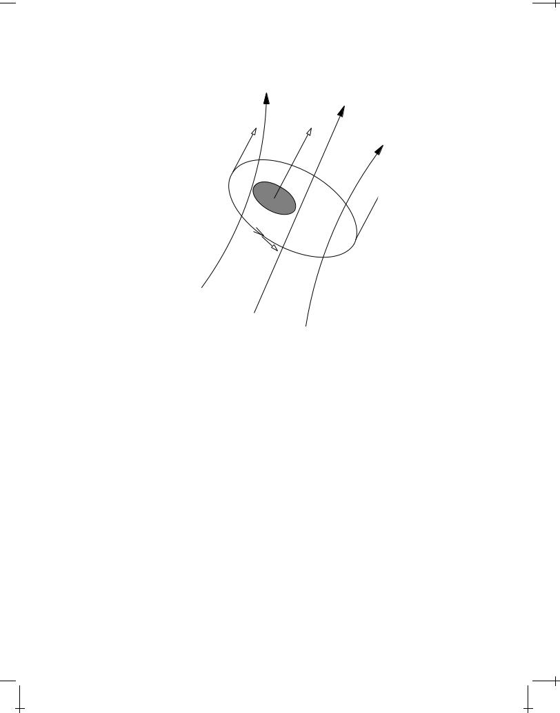
Any change of the magnetic flux m will induce an EMF. Let us therefore consider the case, illustrated if Figure 1.3.4 on the following page, that the “loop” is moved in such a way that it links a magnetic field which varies during the movement. The convective derivative is evaluated according to the wellknown operator formula

dS

v

B(x)

v

C

dl

B(x)

FIGURE 1.3: A loop C which moves with velocity v in a spatially varying magnetic field B(x) will sense a varying magnetic flux during the motion.

which follows immediately from the rules of differentiation of an arbitrary differentiable function f (t;x(t)). Applying this rule to Faraday's law, Equation (1.29) on the previous page, we obtain

(it is one of Maxwell's equations) so that, according to Equation (F.60) on page 155,