electrodynamics / Electromagnetic Field Theory - Bo Thide

or

which leads to the expression

This is the expression to be used in the formulae (8.57) on page 111 for the retarded potentials. The result is (recall that j = v)

For a sufficiently small and well localised charge distribution we can, assuming that the integrands do not change sign in the integration volume, use the mean value theorem and the fact that V dq0 = q0 to evaluate these expressions to become

is the retarded relative distance. The potentials (8.63) are precisely the LiénardWiechert potentials which we derived in Section 5.3.2 on page 63 by using a covariant formalism.

It is important to realise that in the complicated derivation presented here, the observer is in a coordinate system which has an “absolute” meaning and the

x x0

x x0

x(t)

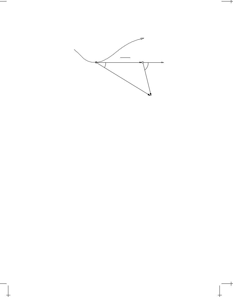
FIGURE 8.3: Signals which are observed at the field point x at time t were generated at the source point x0(t0). After time t0 the particle, which moves with nonuniform velocity, has followed a yet unknown trajectory. Extrapolating tangentially the trajectory from x0(t0), based on the velocity v(t0), defines the virtual simultaneous coordinate x0(t).

velocity v is that of the particle, whereas in the covariant derivation two frames of equal standing were moving relative to each other with v. Expressed in the four-potential, Equation (5.45) on page 62, the Liénard-Wiechert potentials become

The Liénard-Wiechert potentials are applicable to all problems where a spatially localised charge emits electromagnetic radiation, and we shall now study such emission problems. The electric and magnetic fields are calculated from the potentials in the usual way:

8.5.2 Radiation from an accelerated point charge

Consider a localised charge q0 and assume that its trajectory is known experimentally as a function of retarded time

(in the interest of simplifying our notation, we drop the subscript “ret” on t0 from now on). This means that we know the trajectory of the charge q0, i.e., x0, for all times up to the time t0 at which a signal was emitted in order to precisely arrive at the field point x at time t. Because of the finite speed of propagation of the fields, the trajectory at times later than t0 is not (yet) known.

The retarded velocity and acceleration at time t0 are given by

As for the charge coordinate x0 itself, we have in general no knowledge of the velocity and acceleration at times later than t0, in particular not at the time of observation t. If we choose the field point x as fixed, application of (8.68) to the relative vector x x0 yields

The retarded time t0 can, at least in principle, be calculated from the implicit relation

and we shall see later how this relation can be taken into account in the calculations.

According to formulae (8.66) on the facing page the electric and magnetic fields are determined via differentiation of the retarded potentials at the observation time t and at the observation point x. In these formulae the unprimed r, i.e., the spatial derivative differentiation operator r = xˆi@=@xi means that we differentiate with respect to the coordinates x = (x1;x2;x3) while keeping t fixed, and the unprimed time derivative operator @=@t means that we differentiate with respect to t while keeping x fixed. But the Liénard-Wiechert potentialsand A, Equations (8.63) on page 113, are expressed in the charge velocity v(t0) given by Equation (8.68a) and the retarded relative distance s(t0;x) given by Equation (8.64) on page 113. This means that the expressions for the potentials and A contain terms which are expressed explicitly in t0, which in turn is expressed implicitly in t via Equation (8.70). Despite this complication it is

possible, as we shall see below, to determine the electric and magnetic fields and associated quantities at the time of observation t. To this end, we need to investigate carefully the action of differentiation on the potentials.

The differential operator method We introduce the convention that a differential operator embraced by parentheses with an index x or t means that the operator in question is applied at constant x and t, respectively. With this convention, we find that

Furthermore, by applying the operator (@=@t)x to Equation (8.70) on the previous page we find that

(x x0) v @t0

= 1 + c jx x0j @t x

This is an algebraic equation in (@t0=@t)x which we can solve to obtain

where s = s(t0;x) is the retarded relative distance given by Equation (8.64) on page 113. Making use of Equation (8.73) above, we obtain the following useful operator identity

Likewise, by applying (r)t to Equation (8.70) on the preceding page we obtain

which gives the following operator relation when (r)t is acting on an arbitrary function of t0 and x:

With the help of the rules (8.77) and (8.74) we are now able to replace t by t0 in the operations which we need to perform. We find, for instance, that

Utilising these relations in the calculation of the E field from the LiénardWiechert potentials, Equations (8.63) on page 113, we obtain

Starting from expression (8.64a) on page 113 for the retarded relative distance s(t0;x), we see that we can evaluate (@s=@t0)x in the following way

where Equation (8.71) on page 116 and Equations (8.68) on page 115, respectively, were used. Hence, the electric field generated by an arbitrarily moving charged particle at x0(t0) is given by the expression

The first part of the field, the velocity field, tends to the ordinary Coulomb field when v ! 0 and does not contribute to the radiation. The second part of the field, the acceleration field, is radiated into the far zone and is therefore also called the radiation field.

From Figure 8.5.2 on page 114 we see that the position the charged particle would have had if at t0 all external forces would have been switched off so that the trajectory from then on would have been a straight line in the direction of the tangent at x0(t0) is x0(t), the virtual simultaneous coordinate. During the arbitrary motion, we interpret x x0 as the coordinate of the field point x relative to the virtual simultaneous coordinate x0(t). Since the time it takes from a signal to propagate (in the assumed vacuum) from x0(t0) to x is jx x0j=c, this relative vector is given by

where we made use of Equation (8.63) on page 113 and formula (8.74) on page 116. But, according to (8.78a),

The radiation part of the electric field is obtained from the acceleration field in formula (8.81) on the preceding page as

where in the last step we again used formula (8.82) on the facing page. Using this formula and formula (8.86) above, the radiation part of the magnetic field can be written

The direct method An alternative to the differential operator transformation technique just described is to try to express all quantities in the potentials directly in t and x. An example of such a quantity is the retarded relative distance s(t0;x). According to Equation (8.64) on page 113, the square of this retarded relative can be written

If we use the following handy identity

Furthermore, from Equation (8.82) on page 118, we obtain the following identity:

Inserting the above into expression (8.89) on the previous page for s2, this expression becomes

where in the penultimate step we used Equation (8.82) on page 118.

What we have just demonstrated is that, in the case the particle velocity at time t can be calculated or projected, the retarded distance s in the LiénardWiechert potentials (8.63) can be expressed in terms of the virtual simultaneous coordinate x0(t), viz., the point at which the particle will have arrived at time t, i.e., when we obtain the first knowledge of its existence at the source point x0 at the retarded time t0, and in the field coordinate x(t), where we make our observations. We have, in other words, shown that all quantities in the definition of s, and hence s itself, can, when the motion of the charge is somehow known, be expressed in terms of the time t alone. I.e., in this special case we are able to express the retarded relative distance as s = s(t;x) and we do not have to involve the retarded time t0 or transformed differential operators in our calculations.

potentials given by Equations (8.63) on page 113 as follows:

Here 1 = xˆi xˆi is the unit dyad and we used the fact that v v 0. What remains is just to express r in quantities evaluated at t and x.

From Equation (8.63a) on page 113 and Equation (8.96) on the previous page we find that

When this expression for r is inserted into Equation (8.98a), the following result

v v (x x0)[cb c Zc

follows. Of course, the same result also follows from Equation (8.83) on page 118 with v˙ 0 inserted.

From Equation (8.100) we conclude that E is directed along the vector from the simultaneous coordinate x0(t) to the field (observation) coordinate x(t). In a similar way, the magnetic field can be calculated and one finds that