

electrodynamics / Electromagnetic Field Theory - Bo Thide
.pdfM.1 SCALARS, VECTORS AND TENSORS |
163 |
|
A particularly simple rank-two tensor in 3 is the 3D Kronecker delta symbol i j, with the following properties:
i j = k0 |
if i 6= j |
(M.16) |
|
1 |
if i = j |
|
|
The 3D Kronecker delta has the following matrix representation |
|
||
1 |
0 |
0 |
|
( i j) = 530 |
1 |
0 |
(M.17) |
0 |
0 |
186 |
|
Another common and useful tensor is the fully antisymmetric tensor of rank 3, also known as the Levi-Civita tensor
1 |
if i; j;k is an even permutation of 1,2,3 |
(M.18) |
i jk = n0 |
if at least two of i; j;k are equal |
|
ml |
|
|
1 if i; j;k is an odd permutation of 1,2,3 |
|
|
with the following further property |
|
|
i jk ilm = jl km jm kl |
(M.19) |
|
In fact, tensorso |
may have any rank n. In this picture a scalar is considered |
|
to be a tensor of rank n = 0 and a vector a tensor of rank n = 1. Consequently, the notation where a vector (tensor) is represented in its component form is called the tensor notation. A tensor of rank n =2 may be represented by a twodimensional array or matrix whereas higher rank tensors are best represented in their component forms (tensor notation).
In 4D, we have three forms of four-tensor fields of rank n. We speak of
• a contravariant four-tensor field, denoted A 1 2:::n (x ),
• a covariant four-tensor field, denoted A 1 2:::n (x ),
• a mixed four-tensor field, denoted A 1 2:::k (x ).
k+1:::n
The 4D metric tensor (fundamental tensor) mentioned above is a particularly important four-tensor of rank 2. In covariant component form we shall denote it g . This metric tensor determines the relation between an arbitrary contravariant four-vector a and its covariant counterpart a according to the following rule:
def |
(M.20) |
a (x ) g a (x ) |
Draft version released 13th November 2000 at 22:01. |
Downloaded from http://www.plasma.uu.se/CED/Book |
|
|
164
EXAMPLE
M.1
MATHEMATICAL METHODS |
|
This rule is often called lowering of index. The raising of index analogue of the index lowering rule is:
def |
(M.21) |
a (x ) g a (x ) |
More generally, the following lowering and raising rules hold for arbitrary rank n mixed tensor fields:
g |
|
k |
A 1 |
2:::k 1 |
k (x ) = A 1 |
2:::k 1 |
(x ) |
(M.22) |
|
k |
|
k+1 k+2:::n |
k k+1:::n |
|
|
||||
g k k A 1 |
2:::k 1 |
(x ) = A 1 2:::k 1 k (x ) |
(M.23) |
||||||
|
|
|
k k+1:::n |
|
k+1 k+2:::n |
|
|
||
Successive lowering and raising of more than one index is achieved by a repeated application of this rule. For example, a dual application of the lowering operation on a rank 2 tensor in contravariant form yields
A = g g A |
(M.24) |
i.e., the same rank 2 tensor in covariant form. This operation is also known as a tensor contraction.
TENSORS IN 3D SPACE
 nˆ
nˆ
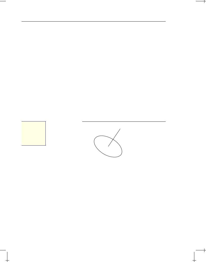
d2x
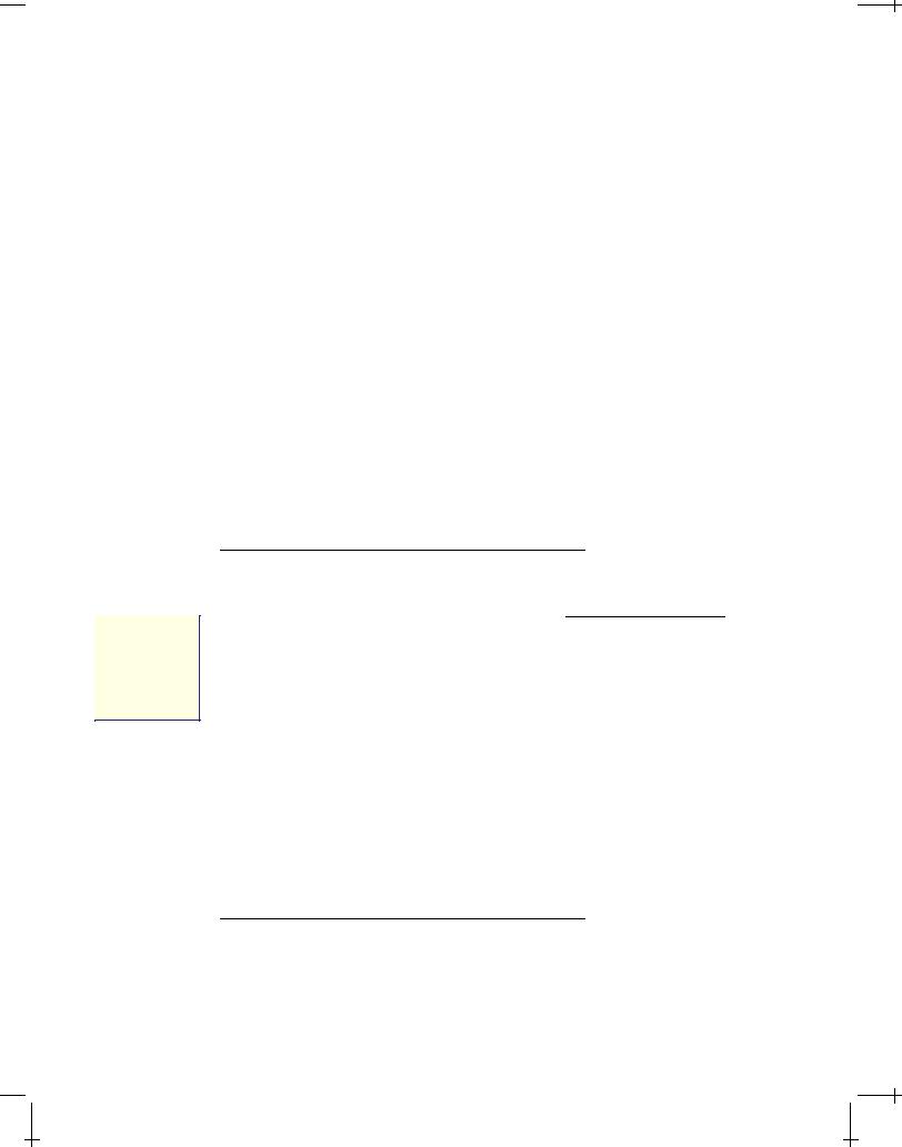
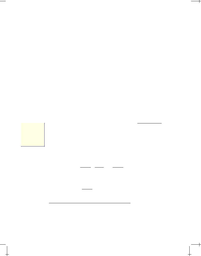
FIGURE M.1: Surface element d2x and the unit normal vector nˆ.
Consider the tetrahedron-like volume element V indicated in Figure M.1 on the next page of a solid, fluid, or gaseous body, whose atomistic structure is irrelevant for the present analysis. Let dS =d2x nˆ in Figure M.1 on the facing page be a directed surface element of this volume element and let the vector Tnˆ d2x be the force that matter, lying on the side of d2x toward which the unit normal vector nˆ points, acts on matter which lies on the opposite side of d2x. This force concept is meaningful only if the forces are short-range enough that they can be assumed to act only in the surface proper. According to Newton's third law, this surface force fulfils
T nˆ = Tnˆ |
(M.25) |
Using (M.25) and Newton's second law, we find that the matter of mass m, which at a
Downloaded from http://www.plasma.uu.se/CED/Book |
Draft version released 13th November 2000 at 22:01. |
|
|
M.1 SCALARS, VECTORS AND TENSORS |
165 |
|
 x3
x3
 nˆ
nˆ
d2x
x2
V
x1
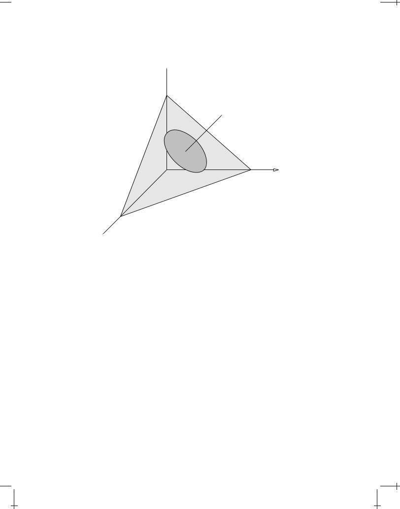
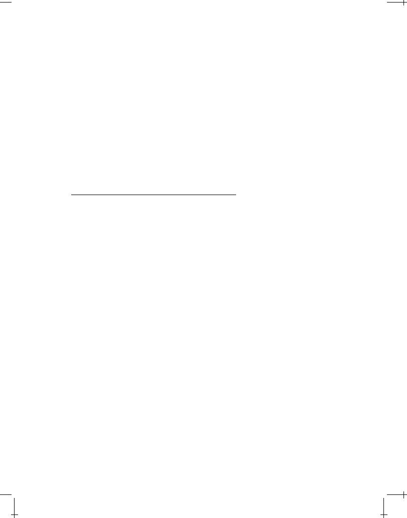
FIGURE M.2: Terahedron-like volume element V containing matter.
given instant is located in V obeys the equation of motion |
|
Tnˆ d2x Txˆ1 d2x Txˆ2 d2x Txˆ3 d2x +Fext = ma |
(M.26) |
where Fext is the external force and a is the acceleration of the volume element. In other words
Tnˆ = n1Txˆ1 +n2Txˆ2 +n3Txˆ3 + |
m |
Fext |
|
||
|
a |
|
|
(M.27) |
|
d2x |
m |
||||
Since both a and Fext=m remain finite whereas m=d2x ! 0 as V ! 0, one finds that in this limit
3 |
|
Tnˆ = åniTxˆi niTxˆi |
(M.28) |
i=1
From the above derivation it is clear that Equation (M.28) above is valid not only in equilibrium but also when the matter in V is in motion.
Introducing the notation |
|
Ti j = =Txˆi > |
(M.29) |
j |
|
for the jth component of the vector Txˆi , we can write Equation (M.28) on the preced-
Draft version released 13th November 2000 at 22:01. |
Downloaded from http://www.plasma.uu.se/CED/Book |
|
|
166 |
MATHEMATICAL METHODS |
|
ing page in component form as follows
3 |
|
Tnˆ j =(Tnˆ ) j = åniTi j niTi j |
(M.30) |
i=1
Using Equation (M.30) above, we find that the component of the vector Tnˆ in the direction of an arbitrary unit vector mˆ is
Tnˆmˆ = Tnˆ mˆ |
|
|
|
3 |
3 |
3 |
(M.31) |
= å Tnˆ jm j = å åniTi j im j niTi jm j = nˆ T mˆ |
|
||
j=1 |
j=1 hi=1 |
|
|
Hence, the jth component of the vector T i jth component of a tensor T. Note that T system used in the derivation.
xˆi , here denoted Ti j, can be interpreted as the is independent of the particular coordinate
We shall now show how one can use the momentum law (force equation) to derive the equation of motion for an arbitrary element of mass in the body. To this end we consider a part V of the body. If the external force density (force per unit volume) is denoted by f and the velocity for a mass element dm is denoted by v, we obtain
|
d |
|
vdm = f fd3x +f Tnˆ d2x |
|
|
(M.32) |
|||
dt fV |
|
|
|||||||
V |
S |
|
|
|
|||||
The jth component of this equation can be written |
|
|
|||||||
|
|
|
d |
v j dm = f f j d3x +f Tnˆ j d2x = f f j d3x +f niTi j d2x |
(M.33) |
||||
|
|
|
|
||||||
fV dt |
V |
S |
V |
S |
|
||||
where, in the last step, Equation (M.30) was used. Setting dm = d3x and using the divergence theorem on the last term, we can rewrite the result as
|
|
d |
v j d3x = f f j d3x +f |
@Ti j |
d3x |
(M.34) |
|||||||
|
|
||||||||||||
fV |
dt |
V |
|
|
V |
@xi |
|
||||||
Since this formula is valid for any arbitrary volume, we must require that |
|
||||||||||||
|
d |
|
|
|
@Ti j |
=0 |
|
|
|
|
(M.35) |
||
|
|
v j f j |
|
|
|
|
|
|
|||||
dt |
@xi |
|
|
|
|
||||||||
or, equivalently |
|
|
|
|
|
|
|
|
|||||
|
@v j |
+ v rv j f j |
@Ti j |
= 0 |
|
(M.36) |
|||||||
|
|
|
|
||||||||||
@t |
|
@xi |
|
||||||||||
Note that @v j=@t is the rate of change with time of the velocity component v j at a fixed point x = (x1;x1;x3).
END OF EXAMPLE M.1
Downloaded from http://www.plasma.uu.se/CED/Book |
Draft version released 13th November 2000 at 22:01. |
|
|
M.1 SCALARS, VECTORS AND TENSORS |
167 |
|
M.1.3 Vector algebra
Scalar product
The scalar product (dot product, inner product) of two arbitrary 3D vectors a and b in ordinary 3 space is the scalar number
a b = xˆiai xˆ jb j = xˆi xˆ jaib j = i jaib j = aibi |
(M.37) |
where we used the fact that the scalar product xˆi xˆ j |
is a representation of |
the Kronecker delta i j defined in Equation (M.16) on page 163. In Russian literature, the scalar product is often denoted (ab).
In 4D space we define the scalar product of two arbitrary four-vectors a and b in the following way
a b = g a b = a b = g a b |
(M.38) |
where we made use of the index lowering and raising rules (M.20) and (M.21). The result is a four-scalar, i.e., an invariant which is independent on in which inertial system it is measured.
The quadratic differential form
ds2 = g dx dx = dx dx |
(M.39) |
i.e., the scalar product of the differential radius four-vector with itself, is an invariant called the metric. It is also the square of the line element ds which is the distance between neighbouring points with coordinates x and x +dx .
INNER PRODUCTS IN COMPLEX VECTOR SPACE
A 3D complex vector A is a vector in 3 (or, if we like, in 6 ), expressed in terms of two real vectors aR and aI in 3 in the following way
def |
def |
ˆ |
3 |
(M.40) |
||
A aR +iaI =aR aˆ R +iaI aˆI |
|
AA 2 |
|
|||
The inner product of A with itself may be defined as |
|
|||||
def |
aI |
def |
|
|
||
A2 A A = aR2 aI2 +2iaR |
A2 2 |
(M.41) |
||||
from which we find that |
|
|
|
|
||
|
|
|
|
|
|
|
A = paR2 aI2 +2iaR aI 2 |
|
|
|
(M.42) |
||
Using this in Equation (M.40), we see that we can interpret this so that the complex
EXAMPLE
M.2
Draft version released 13th November 2000 at 22:01. |
Downloaded from http://www.plasma.uu.se/CED/Book |
|
|
168 |
MATHEMATICAL METHODS |
|
unit vector is
ˆ |
A |
|
|
aR |
|
|
|
|
|
aI |
|
|
|
A = |
|
= |
|
|
|
aˆ R +i |
|
|
|
|
aˆ I |
|
|
|
A paR2 aI2 +2iaR aI |
|
|
paR2 aI2 +2iaR aI |
|
|
|||||||
|
|
|
|
|
|
|
|
|
|
|
|||
|
|
|
aR paR2 aI2 2iaR aI |
|
|
|
aI paR2 aI2 2iaR aI |
3 |
|||||
|
= |
|
|
|
|
aˆR +i |
|
|
|
|
aˆI 2 |
||
|
|
|
aR2 +aI2 |
|
|
aR2 +aI2 |
|
||||||
(M.43)
On the other hand, the definition of the scalar product in terms of the inner product of complex vector with its own complex conjugate yields
EXAMPLE
M.3
jAj2 |
def |
A A =aR2 +aI2 =jAj2 |
|
|
|
|
|
(M.44) |
||||||||
|
|
|
|
|
|
|||||||||||
with the help of which we can define the unit vector as |
||||||||||||||||
ˆ |
|
A |
|
|
aR |
|
|
|
|
aI |
|
|
|
|||
A = jAj |
= p |
aR2 +aI2 |
aˆR +i p |
aR2 +aI2 |
|
aˆ I |
||||||||||
|
|
|
|
|
|
|
|
|
|
|
|
|
|
|
|
(M.45) |
|
|
|
|
aR paR2 +aI2 |
aI paR2 +aI2 |
|||||||||||
|
|
|
= |
|
|
|
|
aˆ R +i |
|
aˆI 2 3 |
||||||
|
|
|
|
a2 |
+a2 |
|
a2 +a2 |
|||||||||
|
|
|
|
|
R |
I |
|
|
|
|
R |
I |
||||
END OF EXAMPLE M.2
SCALAR PRODUCT, NORM AND METRIC IN LORENTZ SPACE
In q4 the metric tensor attains a simple form [see Equation (5.7) on page 54 for an example] and, hence, the scalar product in Equation (M.38) on the preceding page can be evaluated almost trivially and becomes
a b = (a0; a) (b0;b) = a0b0 a b |
(M.46) |
The important scalar product of the q4 radius four-vector with itself becomes |
|
x x = (x0; x) (x0;x) = (ct; x) (ct;x) |
(M.47) |
= (ct)2 (x1)2 (x2)2 (x3)2 = s2 |
|
which is the indefinite, real norm of q4 . The q4 metric is the quadratic differential form
ds2 = dx dx = c2(dt)2 (dx1)2 (dx2)2 (dx3)2 |
(M.48) |
END OF EXAMPLE M.3
Downloaded from http://www.plasma.uu.se/CED/Book |
Draft version released 13th November 2000 at 22:01. |
|
|
M.1 SCALARS, VECTORS AND TENSORS |
169 |
|
METRIC IN GENERAL RELATIVITY |
|
|
|
|
|
|||
|
|
|
|
|
||||
In the general theory of relativity, several important problems are treated in a 4D |
|
|
||||||
spherical polar coordinate system. |
Then the radius four-vector |
can be given as |
|
EXAMPLE |
||||
x = (ct;r; ;) and the metric tensor is |
|
|
M.4 |
|||||
e |
0 |
0 |
|
|
0 |
|
|
|
0 |
e |
0 |
|
|
0 |
(M.49) |
|
|
|
|
|
|
|||||
g = KJI0 |
0 |
r2 |
|
|
0 |
|
|
|
0 |
0 |
0 |
r2 sin2 OLNM |
|
|
|
||
where = (ct;r; ;) and = (ct;r; ;). In such a space, the metric takes the form |
|
|
||||||
ds2 = c2e (dt)2 e (dr)2 r2(d )2 r2 sin2 (d )2 |
(M.50) |
|
|
|||||
In general relativity the metric tensor is not given a priori but is determined by the
Einstein equations.
END OF EXAMPLE M.4
Dyadic product
The dyadic product field A(x) a(x)b(x) with two juxtaposed vector fields a(x) and b(x) is the outer product of a and b. Operating on this dyad from the right and from the left with an inner product of an vector c one obtains
|
def |
ab c |
def |
(M.51a) |
|
A c |
|
a(b c) |
|||
c A |
def |
c ab |
def |
(M.51b) |
|
|
|
(c a)b |
|||
i.e., new vectors, proportional to a and b, respectively. In mathematics, a dyadic product is often called tensor product and is frequently denoted a b.
In matrix notation the outer product of a and b is written
|
a1b1 a1b2 a1b3 |
xˆ1 |
|
||
ab = "xˆ1 xˆ2 xˆ3#53a1b2 |
a2b2 |
a2b3 |
xˆ2 |
(M.52) |
|
|
a1b3 a3b2 |
a3b386 53xˆ386 |
|
||
which means that we can represent the tensor A(x) in matrix form as |
|
||||
a1b1 |
a1b2 |
a1b3 |
|
|
|
"Ai j(xk)#= 35a1b2 |
a2b2 |
a2b3 |
|
|
(M.53) |
a1b3 |
a3b2 |
a3b368 |
|
|
|
which we identify with expression (M.15) on page 162, viz. a tensor in matrix notation.
Draft version released 13th November 2000 at 22:01. |
Downloaded from http://www.plasma.uu.se/CED/Book |
|
|
170 |
MATHEMATICAL METHODS |
|
Vector product
The vector product or cross product of two arbitrary 3D vectors a and b in ordinary 3 space is the vector
c = a b = i jka jbk xˆi |
(M.54) |
Here i jk is the Levi-Civita tensor defined in Equation (M.18) on page 163. Sometimes the vector product of a and b is denoted a ^b or, particularly in the Russian literature, [ab].
A spatial reversal of the coordinate system (x10;x20;x30) = ( x1; x2; x3) changes sign of the components of the vectors a and b so that in the new coordinate system a0 = a and b0 = b, which is to say that the direction of an ordinary vector is not dependent on the choice of directions of the coordinate axes. On the other hand, as is seen from Equation (M.54) above, the cross product vector c does not change sign. Therefore a (or b) is an example of a “true” vector, or polar vector, whereas c is an example of an axial vector, or pseudovector.
A prototype for a pseudovector is the angular momentum vector and hence the attribute “axial.” Pseudovectors transform as ordinary vectors under translations and proper rotations, but reverse their sign relative to ordinary vectors for any coordinate change involving reflection. Tensors (of any rank) which transform analogously to pseudovectors are called pseudotensors. Scalars are tensors of rank zero, and zero-rank pseudotensors are therefore also called pseudoscalars, an example being the pseudoscalar xˆi (xˆ j xˆk). This triple product is a representation of the i jk component of the Levi-Civita tensor i jk which is a rank three pseudotensor.
M.1.4 Vector analysis
The del operator
In 3 the del operator is a differential vector operator, denoted in Gibbs' notation by r and defined as
def |
@ |
def |
|
|
r |
xˆi |
|
@ |
(M.55) |
@xi |
||||
where xˆi is the ith unit vector in a Cartesian coordinate system. Since the operator in itself has vectorial properties, we denote it with a boldface nabla. In “component” notation we can write
@i = |
@ |
; |
@ |
; |
@ |
|
(M.56) |
|
|
@x3 |
|||||
|
@x1 |
@x2 |
|
||||
Downloaded from http://www.plasma.uu.se/CED/Book |
Draft version released 13th November 2000 at 22:01. |
|
|
M.1 SCALARS, VECTORS AND TENSORS |
171 |
|
In 4D, the contravariant component representation of the four-del operator is defined by
@ = |
@ |
; |
@ |
; |
@ |
; |
|
@ |
|
(M.57) |
||||
@x0 |
@x1 |
@x2 |
@x3 |
|||||||||||
|
|
|
|
|
|
|
|
|||||||
whereas the covariant four-del operator is |
|
|||||||||||||
@ = |
@ |
|
; |
@ |
|
; |
@ |
|
; |
|
@ |
|
(M.58) |
|
@x0 |
|
@x1 |
|
@x2 |
|
|
@x3 |
|||||||
|
|
|
|
|
|
|
|
|
||||||
We can use this four-del operator to express the transformation properties (M.13) and (M.14) on page 162 as
y0 = "@ x0 #y |
(M.59) |
and
y0 = "@0 x #y |
(M.60) |
respectively.
THE FOUR-DEL OPERATOR IN LORENTZ SPACE
In q4 the contravariant form of the four-del operator can be represented as
1 |
@ |
1 @ |
|
|
|||||||||||||
@ = |
|
|
|
|
|
|
; @ = |
|
|
|
|
|
; r |
(M.61) |
|||
c |
@t |
c |
@t |
||||||||||||||
and the covariant form as |
|
|
|||||||||||||||
@ = |
1 |
|
@ |
;@ = |
1 |
|
@ |
;r |
(M.62) |
||||||||
c @t |
|
|
|||||||||||||||
|
|
|
c @t |
|
|
||||||||||||
Taking the scalar product of these two, one obtains |
|
||||||||||||||||
1 @2 |
r2 = d2 |
|
|
||||||||||||||
@ @ = |
|
|
|
|
(M.63) |
||||||||||||
c2 |
@t2 |
|
|||||||||||||||
which is the d'Alembert operator, sometimes denoted d, and sometimes defined with an opposite sign convention.
EXAMPLE
M.5
END OF EXAMPLE M.5
Draft version released 13th November 2000 at 22:01. |
Downloaded from http://www.plasma.uu.se/CED/Book |
|
|
172 |
MATHEMATICAL METHODS |
|
With the help of the del operator we can define the gradient, divergence and curl of a tensor (in the generalised sense).
The gradient |
|
The gradient of an 3 scalar field (x), denoted r (x), is an 3 |
vector field |
a(x): |
|
r (x) = @ (x) = xˆi@i (x) = a(x) |
(M.64) |
From this we see that the boldface notation for the nabla and del operators is very handy as it elucidates the 3D vectorial property of the gradient.
In 4D, the four-gradient is a covariant vector, formed as a derivative of a four-scalar field (x ), with the following component form:
EXAMPLE
M.6
@ (x ) = |
@(x ) |
(M.65) |
|
@x |
|||
|
|
GRADIENTS OF SCALAR FUNCTIONS OF RELATIVE DISTANCES IN 3D
Very often electrodynamic quantities are dependent on the relative distance in 3 between two vectors x and x0, i.e., on jx x0j. In analogy with Equation (M.55) on page 170, we can define the “primed” del operator in the following way:
|
@ |
|
|
|
r0 |
= xˆi |
|
= @0 |
(M.66) |
@x0 |
||||
|
|
i |
|
|
Using this, the “unprimed” version, Equation (M.55) on page 170, and elementary rules of differentiation, we obtain the following two very useful results:
r =x |
|
x0 |
j |
>= xˆ |
|
@jx x0j |
= |
x x0 |
= |
|
xˆ |
|
@jx x0j |
(M.67) |
|||||||||
j |
|
|
|
i @xi |
|
j |
x |
|
x0 |
j |
|
i |
|
@x0 |
|||||||||
|
|
|
|
|
|
|
|
|
|
|
|
|
|
|
|
|
i |
|
|||||
|
|
|
|
|
|
= r0 =jx x0j> |
|
|
|
|
|
|
|
|
|
|
|
||||||
and |
|
|
|
|
|
|
|
|
|
|
|
|
|
|
|
|
|
|
|
|
|
|
|
r |
|
1 |
|
|
= |
|
x x0 |
= |
|
r0 |
1 |
|
|
|
|
(M.68) |
|||||||
|
|
|
|
|
|
|
|
|
|
|
|||||||||||||
|
jx x0j |
jx x0j3 |
|
|
|
|
jx x0j |
|
|||||||||||||||
END OF EXAMPLE M.6
Downloaded from http://www.plasma.uu.se/CED/Book |
Draft version released 13th November 2000 at 22:01. |
|
|